| BMI < 18.5 | 太瘦了,要多吃一點 |
| 18.5 <= BMI < 23.9 | 標準身材,請好好保持 |
| 23.9 <= BMI < 27.9 | 喔喔!得控制一下飲食了,請加油! |
| 27.9 <= BMI | 肥胖容易引起疾病,得要多多注意自己的健康囉! |
Python亂談
基礎操作
緒言
語言是跟其他人溝通的工具,顧名思義,電腦程式語言就是跟電腦溝通的話,如果沒有程式,那電腦也就是一堆電子零件罷了。學會語言,可以表達我們的想法,而學會了程式語言後,我們可以要求電腦進行我們想要執行的工作。目前世界上有超過150種的電腦程式語言,就好像一般語言一樣,光是台灣社會常見的就有中文、閩南語、客家話、原住民語(而且各族有各自不同的語言),更不要說其他外語如英文、法文、德文等等。那到底要學哪一種語言比較好呢?首先看是否有特殊需求,例如說你打算跟日本人通商,那當然學日文摟。但若是還沒決定,只是想增加自己的能力專長,那麼一般的選擇就是選最多人學的,也就是最熱門的幾種語言,例如英文。電腦程式語言也是,若沒有特殊目的,可以選擇較多人使用或學習的程式語言,好處是學習資源會較多,通用性也較高,例如C++、Java、Python等等。在這本書中,將介紹Python程式語言並使用該語言來設計程式範例(好吧,這句算是廢話,都說介紹Python了當然使用Python來設計範例。)。我們常說寫程式,總要有個地方讓我們寫,於是有人便設計了合適的編輯器及作業環境方便我們寫程式使用,這樣的軟體稱為IDE(Integrated Development Environment),針對Python設計的IDE有好幾個,在此處使用AnaConda之Spyder,若你電腦中尚未安裝,請參考以下的安裝說明。選擇此IDE的原因是簡單好用容易安裝,首先上網google輸入關鍵字anaconda,即可找到其官方網站,或者直接到以下網址: https://www.anaconda.com/
在anaconda網頁的上方連結列會看到Download,點下去跳到下載頁面。在下方不遠處可以看到以下畫面:
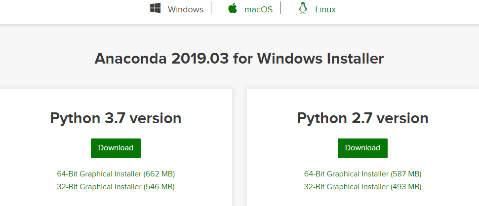 首先選擇Windows、macOS、Linux,看你的電腦是哪一種作業系統,例如是Windows,點選Windows。我們將使用Python 3.7 version(如果有更新的版本,就下載最新版本),至於你的電腦是64-Bit或是32-Bit,可以到控制台(或是Win10的設定)找到系統(Win10是系統>關於)觀察系統類型,便知道是哪種類型,選定之後就點擊下載。
下載完成後,打開檔案總管到下載資料夾,即會看到Anaconda3-xxx-Windows-x86_64.exe類似這樣名稱的檔案,雙擊安裝即可。過程中除非你要更改安裝的位置資料夾,不然只要無腦的按Next即可(或I Agree),應該沒錯的。
花了一段時間後安裝完成,到開始工作列即可找到Anaconda3,如下:
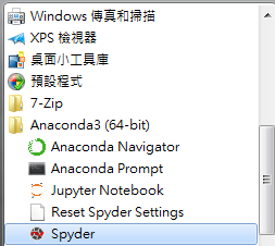
剛才提過Spyder是我們接下來要使用的編譯軟體,可以直接點選開啟。因為會常使用,你也可以在其上點右鍵,選擇釘選到工作列(或開始功能表),之後可以快速開啟。就這樣簡單,開始第一話來閒聊吧!!
第一話、一台大型計算機
電腦原則上是進階版的計算機,顯然它可以比一般的計算機做更多的工作,不過當然它絕對能夠勝任計算機的工作,所以一開始在這裡先漫談如何使用Python進行計算。首先先熟悉一下工作的環境,打開spyder,會看到如下畫面: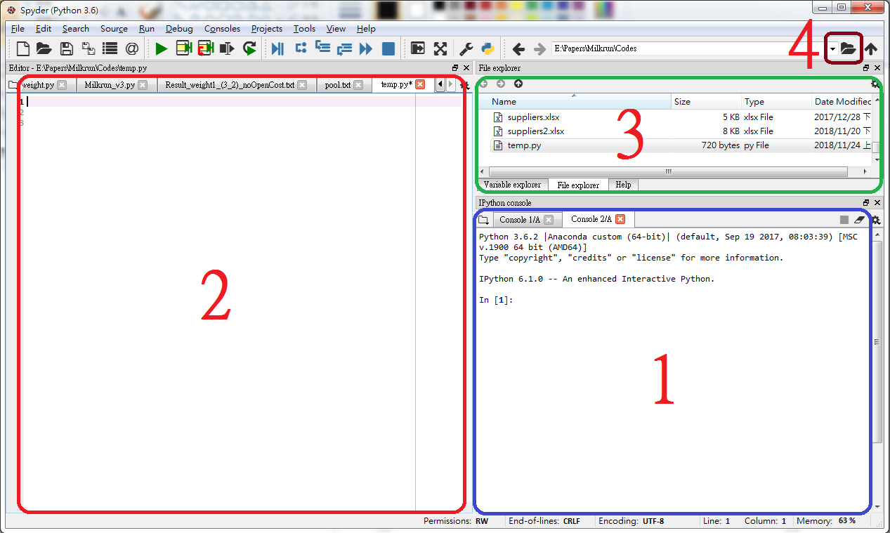
- 右下區塊1稱為console(操縱臺或操作桌),是輸入指令的地方。
- 左邊區塊2是檔案內容編輯顯示區,可以在這裡看到檔案內容或是編輯程式碼。
- 右邊偏上區塊3是下方有三個小按鍵,若是點選左邊的Variable explore,則小視窗中會顯示目前程式的變數及其資料,中間的按鍵是File exploer,會顯示目前資料夾內的檔案,最右邊Help顯示說明資料。
- 右邊偏上區塊4則是檔案總管。
我們要進行計算,可以直接在區塊1,也就是console內輸入即可。所謂一般的計算指的是加減乘除,相信大家都熟到發紫了,雖然若只是要計算加減乘除好像不需要用到這麼豪華的程式,不過程式裡面難免要計算,所以先讓我們來看看怎麼操作。
加減乘除可以直接使用常見的符號,也就是+ (加),- (減),* (乘),/ (除) 等運算子【用來計算的符號稱之為運算子(operator),被計算的數字稱為運算元(operand)】。請注意乘號不是x,要使用*號。輸入算式例如20+5之後,按Enter←鍵即會計算。
20 + 5
20 - 5
20 * 5
20 / 5
不用在意Spyder console內指令前的中括號裡面的數字,那只是在計數輸入了幾次指令,每輸入一次指令,數字便會增加1。 看起來蠻容易的,不過會先乘除後加減嗎?試試看
20 + 5 * 10 / 2顯然是沒有問題。若是有需要先算的部分,跟一般的數學式一樣,使用小括號刮起來就會先計算。例如:
3 * (7 + 8 ) / 6我們來討論一下除法,當某一個數(此時稱為被除數)除已另一個數(此時稱為除數)除或是說用某數(此時稱為除數)除另一數(此時稱為被除數),相當拗口,讓我們簡稱A/B,此時A為被除數B為除數,除了上述的方法直接得到解,若是我們想知道商跟餘數的話,作法如下:
- x // y 符號表示計算x除以y的商數
20 // 3
- x % y 符號表示計算x除以y的餘數 (不是百分比喔)
20 % 3
2 ** 3計算指數時,次方數不一定是整數,也就是說也可以使用例如90.5=3.0。
9 ** 0.5
例題:在平面上有兩個點,其(x,y)座標分別是(5,9)與(18,3),請問要如何使用Python來計算兩點間距離呢?
Answer: 根據距離公式,計算方式如下:
( (5-18)**2 + (9-3)**2 )**0.5
之前看到一個國中的數學題,題目是請問2的2016次方除以13的餘數是多少?使用Python求解的話:
2 ** 2016 % 3我心算了一下,答案為1應該是對的,你可以自己試著解解看。
-
Recap
- Spyder的介紹
- 使用console做數學運算(+、-、*、/、%、**、//)
第二話、變數
變數是做甚麼用的?原則上就是有些資料我們想要特別的記下來,留待之後程式內使用,所以我們跟電腦說,嘿,a等於200,知道嗎?下次我問你a,你就跟我說200。實際上,我們跟電腦借用了一塊記憶體,把這個資料儲存在那塊記憶體內,最重要的是給了這塊記憶體一個名字,下次我們要得到記憶體儲存的資料的時候,就呼叫這個名字,這樣我們就可以得到資料並拿來使用。

例如上圖代表電腦的記憶體,我們使用其中的一塊,讓他幫忙儲存一筆資料,給他名稱為a,讓a指向這個記憶體位置,之後我們只要使用a,就可以指向這塊記憶體並得到儲存在其中的資料。比方說,我們要儲存某人的存款,所以我們在程式中寫a=200,意思是a這個變數就是代表存款,存款的數量就是200。
a=200這個指令稱為變數宣告(variable declaration),舉一反三的同學馬上就想到那是不是能夠說pi=3.14159?當然可以,不過眼尖的同學又發現,咦,一個有小數一個沒有,這樣有沒有差別?答案是有的,差別就是在記憶體中佔據的位元大小。因為我們儲存的資料型態不同,有的時候是整數(int),有的時候是實數(float),這些稱之為變數型態,而其大小則隨著型態而變。好比說我們在一個籃子裏面放水果,放顆荔枝小小空間就可以了,放西瓜就要大一些的空間。
原則上Python中的基本變數型態有以下幾種: 整數(int)、實數(float)、字串(str)、布林(bool) 【布林是直接音譯,說起來總覺得怪怪的,所以之後會直接使用英文boolean表示】,我們可以使用type()這個函數來判定。例如:
a = 200
type(a)
pi = 3.14159
type(pi)
s = "A string"
type(s)
boo = True
type(boo)
在Python中,所有的物件都會給一個編號,通常給的就是記憶體位置,我們可以使用id()這個函數來取得。例如:
id(a)如果你照做了但是得到的id編號跟我的不同,請勿驚訝,我們用的是不同電腦,編號不同是正常的,Python跟你保證你在使用的所有物件都有不同的id,那是因為是不同物件,在不同的記憶體區塊內。
我們可以使用id()這個函數來得到物件的編號,現在說這個做甚麼呢?稍安勿躁,現在我們使用以下指令,讓a=100,然後再檢查id(a),得到如下結果:
a = 100
id(a)
咦,a的id編號變了,我們不是把a內的值改變了嗎?其實不是,而是我們讓a指向另一塊記憶體了,而這塊記憶體儲存的值是100。現在我們再定義b=200,然後再看看b的id,如下:
b = 200
id(b)
咦,b的id跟剛剛a等於200的時候id相同。原來情況是這樣,再借用剛剛的記憶體的圖如下,剛開始a指向記錄著200的記憶體,然後我們又讓a指向記錄著100的記憶體,接著我們換讓b指向記錄著200的記憶體。也就是說我們沒有修改記憶體中的數值,只是讓變數在記憶體中變換指向的記憶體區塊片段。

這等行徑與其他語言大相逕庭,例如C++,他們的做法是修改記憶體的儲存內容,變數倒是指向同一個記憶體。
上述的解釋說明了Python宣告變數的動態型態。跟其他許多程式語言不同的地方是,當我們在宣告變數的時候,並不需要告訴Python我們現在要宣告甚麼型態的變數,程式自然會根據你給的數值來判定,而當我們改變數值甚至型態時,Python會將此變數指位到另一個記憶體區塊,從而改變其數值及型態。例如我們將上述的a=3.14159,然後再檢查它的變數型態跟編號,結果如下:
a = 3.14159
type(a)
id(a)
可以看到a的型態變成了實數(float),而且id編號也完全不同了。也就是電腦先找了一塊記憶體,存了3.14159這個float數值在裡面,然後等著a來指位。說了半天,重點是當我們在Python中宣告變數的時候,不需要給定變數的型態。
-
Recap
- Python變數的宣告(不需給變數型態)及其在記憶體中的關係
- 使用id()求得編號,使用type()得到變數型態
第三話、變數的操作
變數既然都被稱之為數了,那拿來計算應該沒甚麼問題。那我們來試試看。a = 200 a * 3 a + 100確實可以計算,不過怎麼看起來怪怪的,a不是已經變成600了嗎?怎麼+100之後又顯示300。原因是在console裡面這樣計算並沒有改變a的值,只是顯示答案給我們看而已,若要改變a所代表的值,我們需要讓它等於a才行。所以我們先學習一個觀念,就是等號的意義。
在程式中的等號(=)意義並不是相等,而是指派(assign)。意思是將等號右邊的數值,指定給左邊的變數。所以我們不能使用10 = x。也不能使用 x + y = 10,因為等號左邊只能有一個變數名稱。 完成之後,在電腦的記憶體內,10這個數字儲存在x對應的記憶體中。之後我們可以隨時將其取出。
這樣大家清楚了,所以若是我們要讓a的值真的改變(事實上是a所指向的記憶體改變,在上一話大家應該都清楚了),應該如下操作。a = a * 3 print(a) a = a + 100 print(a)a = a + 100這樣的指令讓我們難受,因為跟平常學的數學用法完全不同,所以我們可以如此理解:先將等號右邊的計算好(例如a是600,a+100得到700),然後將算出來的值指派給等號左邊的變數名稱(所以此時a等於700)。
好吧,這個觀念是最基本的,學寫程式的人一定要懂,但是也不難,我想你現在一定懂了,讓我們繼續看下去。
我們之前提到基本的變數型態包含整數(int)、實數(float)、字串(str)跟布林(bool),整數實數拿來運算沒有問題,那麼字串呢?看一個例子。
s = "我是字串"
print(s*3)
print(s+3)
這次的變數主角叫做s,它的值是"我是字串",很明顯它是指向一個字串。咦,字串乘以3,這樣也行?是的,字串如果乘以3,表示將3個相同字串串接在一起。但是字串+3不行嗎?不行,我們看到最後顯示了一行
TypeError: must be str, not int這是甚麼意思?意思是說,變數型態錯誤,必須是字串,不是整數。白話文就是說字串可以加字串,但是不能加整數。所以如果我們真的想讓字串+3的話,可以如下方式:
s + "3"或許你會好奇,字串可以+跟*,那可以使用-跟/嗎?你可以自己試試看,答案當然是不行。
好吧,那麼boolean呢?首先我們先了解一件事情,那就是boolean只有可能有兩個值,True(真)跟False(偽)【請記得在Python中,這兩個值的第一個字母要大寫】。簡單吧,看以下例子:
b1 = True
b1 * 3
b2 = False
b2 * 3
咦,發生甚麼事,為何一個是3,一個是0。原來在Python中,True的值用1代表,False的值用0代表,所以會產生這樣的結果。
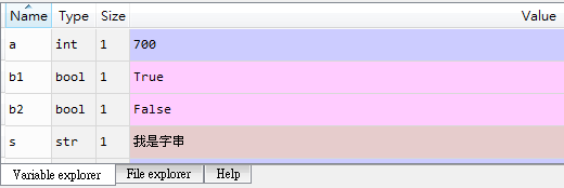
順帶提一下,在Spyder中建立的變數,都會記錄在Console上方Variable explorer視窗中,你可以在其中看到變數的名字型態跟值。
-
Recap
- 變數的使用及計算
- 字串使用*號表示複製次數
- True(1)與False(0)首字母需大寫
第四話、命名
之前提過變數要有一個名字來表示,也就是說每一個變數我們必須幫忙取名,事實上變數之外的函數或物件也都要取名,這跟給人取名一樣,有一些禁忌跟常規,一般命名的規則如下:- 可以使用數字與英文字還有底線來命名,例如a, x1, x_1。
- 名稱的第一個字母不可以是數字,例如2a是不允許的。但是可以是底線,所以_2a是可以的。
- 名稱中不可包含空白(space 或 tab),例如 x y = 10是不可以的,若是使用會出現錯誤。
- 可以使用大寫,大寫跟小寫是不同的。例如a=5與A=5代表兩個不同的變數。不過一般變數名稱命名習慣是使用小寫字母開頭,物件是大寫字母開頭。
- 通常使用有意義的英文字來表示變數,例如age = 12。若是需要兩個以上的英文字,則後面的字首用大寫來區分,例如myAge = 12。也有得人喜歡用底線區分,例如my_age = 12。在一個程式中,可能會有許多意義相差不大的變數,現代的命名慣例,希望程式設計師盡量取個可以明白表示意義的變數名稱,即使會讓變數名變很長都沒關係,例如:travelCostOfDeliveryTruck, travelCostOfCollectionTruck。
- 不要使用關鍵字來命名。例如使用for = 5。Python的關鍵字取得方式如下:
import keyword
print(keyword.kwlist)
['False', 'None', 'True', 'and', 'as', 'assert', 'async', 'await', 'break', 'class', 'continue',
'def', 'del', 'elif', 'else', 'except', 'finally', 'for', 'from', 'global', 'if', 'import', 'in',
'is', 'lambda', 'nonlocal', 'not', 'or', 'pass', 'raise', 'return', 'try', 'while', 'with', 'yield']
- 盡量避免與內建函數同名,雖然程式可能還是會執行,但是容易造成混淆,且之後可能產生錯誤。例如使用type = 1。
- 理論上可以使用中文來當作變數名稱,但是強烈建議不要如此使用。例如:
哆啦A夢 = "機器貓""
- 不要使用特殊符號命名,例如#@$。
@@ = "驚訝"

你可以觀察到幾個函數例如__call__(), __delattr__(), __dir__()等等,都是前後有兩條底線,這樣的函數名稱是Python的習慣用法,我們在做類似定義時要注意。那們可以這樣命名嗎?
___ = "臉上三條線"
____ = "臉上四條線"
print(___)
print(____)
應該是沒有違反規則,很難跟你說不行,不過我很擔心十八條線的情況,所以別再做奇怪的事(咦,那我剛才在做甚麼?___)。
-
Recap
- 了解變數與函數的命名規則及慣例
- 使用help()查詢資料
第五話、cast
之前提過變數各有形態,有的是數字,有的是字串。那形態之間能夠轉換嗎?答案是肯定的。我們只要使用內建函數int(), float(), str(), bool()即可將不同形態的變數變成另一個形態,這個指令稱為cast。例如:s1 = '3' s2 = '9' print(s1+s2)這個例子中,s1跟s2都是字串,但是內容看起來是數字,我們若將兩者相加,會變成字串+字串,結果是兩個字串串在一起,如果我們想要的是數字相加,那我們需要先將字串轉換成數字,如下:
int(s1) + int(s2)使用int(s1)來將字串s1轉換成為int。當然int也可以使用str()來轉成字串。再看下一個例子:
s3 = "10"
float(s3)
將字串變成float,看起來是OK的,那如果我們這麼做呢?
s4 = "3.14159"
int(s4)
這樣就出現錯誤了,因為3.14159這個字串,沒有辦法變成整數。那如果本來是個實數呢?
f = 3.14159
int(f)
看起來我們只能取得整數的部分。之前我們說過boolean中的True是用1表示,False是用0表示,現在我們將其轉換成整數看看。
int(True)
int(False)
嗯哼,果然沒錯。
-
Recap
- 轉換變數型態,使用int()、float()、bool()、str()
第六話、字串
其實在之前我們已經用了字串了,原則上就是文字,但是為了怕跟其他的程式內容混淆,所以用雙引號括起來,表示這是字串,不是其他東西。不過事實上在Python中表示字串的方式有以下幾種:str1 = '我是字串,兩邊各一撇' str2 = "我也是字串,兩邊各兩撇" str3 = '''Me too,兩邊各三個一撇''' str4 = """Me three,兩邊各三個兩撇"""好吧,不管用一個一撇,一個兩撇,三個一撇,或是三個兩撇,都算是字串。為何要搞這麼多種,難道是特別要混淆我們嗎?其實三撇的字串是有不同,就是他們可以跨行,也就是兩個三撇之間的全部都是字串。
"""
abc
def
ghi
"""
'''
do re mi
fa so la
si do
'''
出現的\n是換行的意思,在之後說明。
此外,Python字串可以顯示Unicode字元,甚麼是Unicode?在一開始有電腦的時候,只需要能夠使用數字跟26個英文字母就行了,畢竟第一台電腦是美國人發明的(也有其他國家的科學家建立一些原始型態的大型計算機,在此就不深究),但是等發展較為成熟了,其他國家的人也能使用後,就出現了希望在電腦內使用其他語言的需求。26個字母(大小寫不同)加數字不多,短短的記憶體就能表示完畢,但是像中文字,單字的數量龐大許多,再加上其他語言例如日文韓文泰文法文希伯來文等等,為了讓全球的人都能夠使用電腦,於是制訂了unicode編碼,把所有語言都收錄,經過多次更新改版,收錄了13萬多的文字符號,使用16進位法表示。在Python中可以直接使用\u開頭加上碼位(code point)組成來顯示,中文的話主要介於4E00~9FBB之間。例如:
"\u6001\u6002\u6003"
"\u6aaa\u6bbb\u6ccc"
也可以顯示日文,例如:
"\u3042\u3043\u3044\u3045\u3046"或是韓文等。
"\uc5fd\uc5fe\uc5ff"雖說可以這樣顯示文字,但是不可能記下來,作業系統有自己的編碼(例如Windows的記事本應該是MS950),所以要輸入中文只要使用中文輸入即可,在Python(3.x)中,str就是unicode。
type(u'a')
type(b'a')
前面加上u就是表示是unicode,而加上b表示是位元組(bytes)編碼。我們可以使用encode()函數來取得不同編碼內容。例如:
u8 = '小叮噹'.encode('utf-8')
print(u8)
b5 = '小叮噹'.encode('Big5')
print(b5)
若想要知道一個字的unicode,可以使用ord()函數。若想知道一個數字(十進位)所代表的文字符號,則使用chr()函數。例如:
ord('電')
chr(38651)
hex()函數可用來將十進位數字轉換成十六進位。
hex(38651)本來若是要在程式中加入中文,需在前面加上# -*- coding: utf-8 -*-這一行來表示其編碼形式為utf-8,才可正確顯示,不過在Python 3.x版本中,已經預設為utf-8,所以應該都可正常顯示。
-
Recap
- 單行字串與多行字串
- unicode的介紹與使用以及使用encode、ord、chr等函數
第七話、print()
print()函數的意義就是顯示資訊,之前已有使用過,看一下它的help。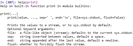
嗯,好吧,可以印出value。算了,還是直接給例子。
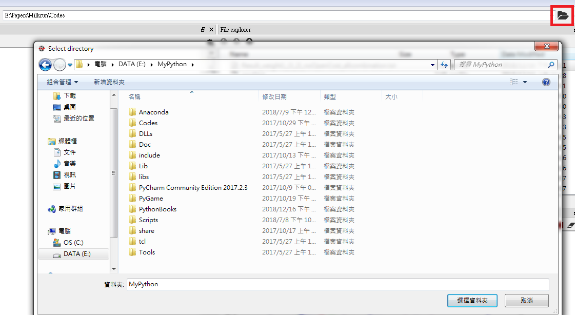
print("Hello, World!")
print(3+3)
原來可以顯示小括號內的內容,不過等等,沒有使用print()不是也會顯示嗎?在console是沒有問題,但是在程式檔案內就不一樣了。現在來試一下,首先在右上方的路徑列選擇你要將檔案放置的資料夾位置,你可以使用旁邊的資料夾圖樣操作。
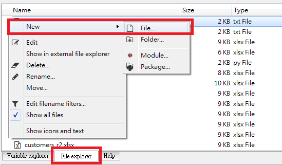
選擇了之後,可以在File explorer的空白處點右鍵,然後開啟新檔案。或是直接開啟新檔案,之後再儲存到目標資料夾即可。
接著在左邊的檔案中,輸入3+3,將檔案儲存為py1.py(因為是python檔案,所以延伸檔名須為.py),然後在上方的下拉選單裝找到Run>Run,或是直接按F5,或是在上方快捷按鈕找到最大的綠色三角形(你不可能會錯過它),點下去即可執行。
執行之後你會在console看到類似如下的顯示:

你的檔案路徑可能跟我的不同,不過這表示執行完成了。不過剛剛打的3+3呢?沒看到結果,顯見這樣是無法看到解,現在再到檔案處改為print(3+3)然後在執行一次。耶,有了,所以結論是如果在console,有沒有print()都會看到結果(其實他們呼叫的是不同方法,這在後面再提),在檔案內,一定要用print()才能顯示。
再來就簡單了,再試一下其他的。
cars = 2
print("Tom has " + cars + " cars.")
挖哩,這樣不行嗎?嗯,這個錯誤似曾相似,字串+數字確實是怪怪的,想起來要把數字cast成字串了。
print("Tom has " + str(cars) + " cars.")這樣好多了。不過老是cast有點麻煩,沒關係,Python還提供另一個較簡單的寫法。
print("Tom has", cars, "cars.")蠻好的,不過跟上面的有一些些不同,原來在使用逗點連結時,會自動幫我們加上一個空白,所以如果你跟之前一樣留字間空白,反而會得到兩個字間空白。再來:
name = "A"
height = 1.293
weight = 129
print(name, "的身高是", height, "公尺,體重是", weight, "公斤")
好像逗點有點多,而且有點想把身高顯示個兩位就好了,於是發展出了格式化字串(format string),那要怎麼做呢?一開始套用C語言的語法,如下:
print("%s%的身高是.2f公尺,體重是%d公斤" % (name, height, weight))
嗯,%s意思是這裡放字串(str),%.2f意思是這裡放小數後兩位的實數(float),%d表示這裡放整數,後面的百分比號表示之後的內容一一對應到前面字串內的內容,也就是name對應到%s,height對應到%.2f,而weight對應到%d。好吧,本來這樣也行得通,不過%號總覺得不太親民,所以後來又修改為:
print("{}的身高是{:.2f}公尺,體重是{}公斤".format(name, height, weight))把中間的%改為文字format,也就是說format()是字串的方法,然後字串內要加入變數的地方用{}代替%x,嗯,看來簡潔且好理解多了,小數後兩位還是.2f,只是前面加個冒號(:)來表示要做處理。這個例子中的format()內有三個變數,事實上他們依序對應的參考號碼為0,1,2,甚麼意思呢?就是如果我們在字串內的{}中加入參考號碼,就可以將對應的變數顯示在那個位置。看一下下例。
print("{1}的身高是{2}公尺,體重是{0}公斤".format(name, height, weight))用這個方式可以將變數顯示在想要的位置,不過會不會瞄準錯位置?好吧,親愛的,如果你不小心記得了上面兩個format string的方法,現在你可以把他們忘了,現在更新的顯示方法出來了,叫做f-string,用法如下:
print(f"{name}的身高是{height:.02f}公尺,體重是{weight}公斤")是不是更容易了?只要在字串前面加個f就完成了,也不需要再瞄準那個對應哪個了,直接將變數寫到{}內即可。這招我們一定要學會。
-
Recap
- 使用print()函數來印出資料內容
- 使用+、,、%、format()、以及f-string(f"")來印出文字與變數
第八話、Escape Characters
Escape character有些翻譯為逸出字,嗯,翻譯似乎讓我更為迷惘。假設我們想要顯示出如下文字訊息>>我真是"帥"啊。這要怎麼做?print("You are "so" beautiful.")不行,有錯,看到帥變成黑的就覺得不太對。原來兩個"之間電腦會將其視為一個字串,所以碰到帥前面的",電腦就將其當成另一個"來形成字串了,可以我想要把"印出來,電腦怎麼可以放過它呢?是有方法的,就是給他一個記號,跟電腦說這個”是有其他涵義的,你跳過它吧,好吧,程式語言的設計者找了半天,終於找到一個比較少用的符號,那就是\。也就是說只要我們把\加在特殊的字元前面,例如",就是代表這次的"不再是字串的一端了。試試看。
print("You are \"so\" beautiful.")嘿,可以了。不過事實上Python做這件事情可以使用另一個方式,記得之前我們說形成字串的幾個符號,因為我們想要印兩撇,那麼我們就使用一撇來表示字串就好了,這樣電腦就不會搞混了。
print('You are "so" beautiful.')雖然這解決了”的問題,卻也不代表\不需要使用了。例如如果我們想要打出\符號的話怎麼辦?因為我們已經設計使用\來表示特殊字元,所以當電腦看到\的時候,心中會猜疑是不是後面接了甚麼特殊字元要打印出來,反而不會想到是要印出\符號,所以如果要印出\符號的話,我們可以在它之前再加上一個\符號,表示這個\是特殊字元,是不是很拗口?看看結果如下:
print("\\")完美。除此之外,還有那些escape characters?
- \t: tab,相當於4個空白
- \n:new line,換新行
- \':打出單引號,跟\"意思類似。
- \u:unicode,之前使用過的,16bit十六進位值
- \ooo:ooo的八進位值所表示的字元,例如: "\101"
-
Recap
- 在字串中加入escape characters(使用符號\)
第九話、if跟relational operators
在程式中需要判斷在某些情況下做甚麼事情,就好比說洗衣機,有的會判斷如果衣服多一些,那就用水多一些。這個時候,我們需要if statement,語法如下:
首先我們看到需要使用關鍵字if,後面接著一個條件(condition),這個白話翻譯就是如果某個條件為真,那麼就做甚麼(do something)。在這個格式中,condition後面需要有一個冒號,而do something前面需要右縮(indent)。這是Python的固定格式,do something可能是需要好幾行的指令,為了讓電腦知道哪一些指令是在condition為真後要做的事情,所以讓這些指令,無論是幾行,往右縮排,這樣電腦就知道這些事要做的事情。在其他程式語言例如Java,則是使用大括號來將要做的事情包含。不過通常為了程式碼顯示格式清除,一般即使Java我們也希望程式設計員有縮排,所以Python的設計理念乾脆把不用括號,直接以縮排來表示要被執行的指令,少了括號也看起來比較不那麼亂,而且括號常常會括錯,反而造成其他的錯誤。
至於往右縮排多少,原則上是一個Tab(四個空白),在Spyder中,只要在輸入:後,按下Enter,程式就會自動幫我們往右縮一個Tab了,這個功能可以多利用。接著我們要看Condition,原則上這個condition就是boolean,也就是True跟False。也就是說我們可以這樣做。
if True:
    print("真的")
這樣是可以的,不過這其實是脫褲子放屁,多此一舉。因為既然不需要說如果,本來就會印出,如果為真,當然也會印。那如果我們把True改為False呢?Well,那就是白費力氣了,因為是False,所以根本就不會執行。因此,我們不會在if後面直接寫上True或是False,而是根據某些判斷而來,所以接下來介紹關係運算子(relational operators)。
關係運算子可以用來判斷兩數的關係,包含:
- A==B(A等於B?)
- A>B(A大於B?)
- A<B(A小於B?)
- A>=B(A大於等於B?)
- A<=B(A小於等於B?)
- A!=B(A不等於B?)
現在我們來看個例子。
大雄媽媽說如果數學成績及格,會給大雄額外的零用錢,大雄數學考50分,會拿到額外零用錢嗎?
math = 50
if math >= 60:
    print("有額外零用錢")
Oops!看起來甚麼都沒拿到。
通常我們說如果怎樣,否則的話,就怎樣。我們可以加上否則嗎?答案是肯定的,在Python中,使用關鍵字else來表示否則。首先我們要先了解,我們會說如果怎樣,否則就怎樣,但是如果沒有說如果,我們不會只說否則怎樣,但是我們可以說如果怎樣,不一定要說否則就怎樣(希望你有看懂,)。這在程式中也是一樣的,我們可以使用if但不使用else,也可以使用if加上else,但是不可以僅使用else而沒有if。看一下if…else…的語法架構。
if Condition:
    Do something 1...
    Do something 2...
else:
    Do other thing 1...
    Do other thing 2...
這樣應該很清楚了,如果使用if…else…,if之下的程式碼是在情況為真時執行,而else之下的程式碼則是在情況不為真的時候執行,所以else不需要條件,直接打上:號就可以了。這一定要記得,千萬不要給else條件了,它的條件就是if後面的條件不為真的情況。再來看個例子:
大雄媽媽說如果數學成績及格,會給大雄額外的零用錢,但是如果不及格的話,這個月就沒有零用錢,大雄數學考50分,會發生甚麼事?
math = 50
if math >= 60:
    print("大雄拿到額外零用錢")
else:
    print("大雄這個月沒有零用錢")
這次我們將程式碼寫在檔案內,按下執行(F5)後,你就會看到結果了☺。
-
Recap
- if statement語法介紹
- 使用關係運算子(==、>、<、>=、<=、!=)來判斷兩數關係
第十話、再說if跟Logical operators
之前提到if...else...可以判斷兩個情況(True跟False),決定在不同情況做不同的處置,那如果我們有三個情況呢?比方說:大雄媽媽說如果數學成績及格,會給大雄額外的零用錢,但是如果不及格的話,這個月就沒有零用錢,但若是考超過90分,就帶他出去度假。
這問題有三個條件,分別是超過90分,介於90跟60間的分數,以及低於60分。在這三個條件下,分別有對應的動作。那我們還可以使用if…else…來判斷嗎?當然是可以,如下:math = 50 if math >= 90: print("全家去度假") else: #這裡分數小於90 if math >= 60: print("大雄拿到額外零用錢") else: print("大雄這個月沒有零用錢")最左邊的if…else…是一套的,如果if成立,表示分數大於等於90,如果不成立,表示進入到else,而這裡的條件是分數小於90。而在else之下,又有一組的if…else…,我們已知在這裡分數肯定小於90,所以判斷如果大於等於60為真,否則就是小於60。這樣的方式可以處理3個情況。
額外一提的就是#字號,若是加上這個符號,表示從這個符號開始到這一行結束,都是註解(comment),註解的意思就是做個解釋,這個解釋是給我們自己看的,不是給電腦程式看的,所以電腦不會執行它,會直接跳過。
好吧,聰明如你,一定聯想到了如果有四個甚至五的條件的時候要怎麼做了,我們只要在else裡面再加上if…else…一路追加下去就可以了。雖然這好像是沒有問題,不過當一層一層往下之後,會變得越來越複雜,於是Python提供另一個方式來簡化這個情況,就是提供另一個關鍵字elif,其實elif原則上就是else if的縮寫。我們重寫上例來說明。
math = 90
if math >= 90:
    print("全家去度假")
elif math >= 60:
    print("大雄拿到額外零用錢")
else:
    print("大雄這個月沒有零用錢")
這個if…elif…else…的組合,可以讓我們判斷三個不同的情況,如果是四個情況,就是if…elif…elif…else…,簡單吧。要記住的是,只要包含了if(也就是if跟elif),就必須要給條件,再次強調,else是不需要也不能給條件的。
在之前的例子中,給的條件都是單一個boolean值,若是同時要考慮多個boolean值要怎麼做呢?首先這是甚麼意思,何謂考慮多個boolean值?先看以下例子:
大雄媽媽說如果數學成績及格,而且英文也及格,會給大雄額外零用錢,若是只有一科及格,一科不及格,那就不多給零用錢,但是如果兩科都不及格的話,這個月就沒有零用錢。
這個問題會牽扯到三個狀況,數學及格英文也及格,數學英文有一科及格一科不及格,兩科都不及格。這時候怎麼辦?在程式設計中,此時要使用Logical operators,白話翻譯是邏輯運算子。當數學及格英文也及格的情況發生,表示數學大於等於60是True,英文大於等於60也是True,此時我們用and關鍵字。當使用and運算的時候,and的兩端是boolean,而這個運算會傳回一個boolean,and的運算結果若為True,表示其兩端都是True。(True and True are True.)
我們先在console測試一下。
math = 60
eng = 70
math >= 60 and eng >= 60
只要有一科不及格,那麼math >=60 and eng>=60就會傳回False。
那麼只有一科及格,要怎麼傳回True?此時要使用關鍵字or。使用or運算子時,一樣兩端都是boolean,運算完傳回一個boolean,傳回True的條件就是兩端至少有一個是True。也就是說,只有兩端都是False的時候,才會傳回False,其他都會是True。這次直接用True跟False測試看看。
True or False
False or False
好吧,學會了這兩個來解決剛剛的問題就足夠了,寫法如下:
math = 65
eng = 65
if math >= 60 and eng >= 60:
    print("大雄拿到額外零用錢")
elif (math >= 60 and eng < 60) or (math < 60 and eng >= 60):
    print("大雄沒有拿到額外零用錢")
else:
    print("大雄這個月沒有零用錢")
一科及格一科不及格的情況下,我們需要列出數學及格且英文不及格還有英文及格且數學不及格的兩個狀況,兩者任一都是True,所以使用or。這樣有點麻煩,所以Python還提供另一個語法,叫做xor,意思是只要運算子的兩端一個是True,一個是False,這樣會傳回True,如果都是True或是都是False,那就傳回False,使用的是符號^,還是先測試一下。
True ^ True
True ^ False
False ^ True
False ^ False
乾脆一點都列出來了,現在我們可以重寫上面的程式碼,讓它看起來簡潔一點。
math = 55
eng = 65
if math >= 60 and eng >= 60:
    print("大雄拿到額外零用錢")
elif math >= 60 ^ eng >= 60:
    print("大雄沒有拿到額外零用錢")
else:
    print("大雄這個月沒有零用錢")
最後再介紹一個邏輯運算子,就是not。這個運算子跟之前不同的是它沒有兩端的運算元,它的主要目的就是否定原來的boolean,使其True變False,False變True。一樣測試一下。
not True
not False
好吧,Easy-peasy。雖然不需要,但是如果硬要將not用到上面的例子,我們可以這樣寫。
math = 66
eng = 65
if not math < 60 and not eng < 60:
    print("大雄拿到額外零用錢")
elif math >= 60 ^ eng >= 60:
    print("大雄沒有拿到額外零用錢")
else:
    print("大雄這個月沒有零用錢")
not math < 60的意思就是數學不是小於60,那就是大於等於60摟。也就是說,如果math<60是False,那麼加上not就變成True。
現在各位應該都熟悉了邏輯運算子了,來練習以下的例子。
weight = 45
height = 1.62
bmi = weight/height**2
if bmi < 18.5:
    print(f"bmi={bmi},你太瘦了")
elif bmi < 23.9:
    print(f"bmi={bmi},你是標準身材")
elif bmi < 27.9:
    print(f"bmi={bmi},你要控制一下飲食了")
else:
    print(f"bmi={bmi},肥胖容易引起疾病")
順道提一下,如果要判斷某數是否介於某一個範圍,例如:
a = 5
a > 1 and a < 10
理論上這樣寫是絕對沒有問題的,不過Python提供更簡單的語法:
1 < a < 10跟我們平常寫的數學是一樣的,很酷吧!
-
Recap
- 多重狀況的if…elif…else…語法
- 使用邏輯運算子and、or、not運算兩個boolean
第十一話、指派運算子
之前我們提過=是指派的意思,我們需要先將等號右邊的值算出來,再將這個值指派給等號左邊的變數,例如:a = 1 a = a + 1 print(f"a = {a}")程式設計師最喜歡將程式碼簡短化,我猜測應該是打字太多手會痠,所以他們花費了好幾個小時,終於想到了將上面的指派方式簡化,變成如下方式:
a += 1 print(f"a = {a}")是不是變得簡短許多?(好像還好,,不過如果不是a,而是一個名字很長的變數,就會比較有感覺了)。a+=1與a=a+1兩式的意義完全相同,你可以任選一個,+=這個符號稱為指派運算子。
聰明的你一定想到了如果要運算的不只是+,是不是有其他的指派運算子?答案是肯定的,除了+=之外,還有-=、*=、/=、**=、//=、%=,你可以自己練習看看。
-
Recap
- 符號=用於指派變數的值
- a = a+1等同於a+=1
第十二話、本體運算子
之前我們學過使用==來判斷兩者是否相同,==的相同含意是值相同,例如:a = 1 a == 1這個部分沒有問題,不過下面的例子就奇特了。
True == 1
5 == 5.0
True == 1.0
這幾個例子都是傳回True,不過==兩邊的形態都各不相同,這在我們需要考慮兩個變數是否相同型態時會出現誤判。所以如果我們想要知道兩者是否形態跟值都相同的情況下,我們應該使用關鍵字is,此稱為本體運算子(Identity operator)。例如:
True is 1
int(True) is 1
只有在相同型態且相同值才會傳回True。如果是要判斷是否不同呢?此時可以借用之前學過的關鍵字not,例如:
not int(True) is 1 int(True) is not 1兩個方式似乎都可以,不過第二種方式比較像英文,感覺自然一點,自然就是美,是吧☺!
-
Recap
- 符號==用來判斷值是否相同
- 關鍵字is用來判斷值與型態是否相同
第十三話、運算優先順序(Operators Precedence)
我們已經學會了好幾種運算子,跟數學一樣,有時候會組合成一個式子其中包含多個運算子,此時的運算先後次序是甚麼呢?從小我們就知道先乘除後加減,那程式的運算是否也遵循類似的規則呢?答案當然是的,這些運算子的優先順序如下:| 優先順序 | 運算子 |
|---|---|
| 1 | ** |
| 2 | ~ ,+, - |
| 3 | * ,/, %, // |
| 4 | +,- |
| 5 | >>, << |
| 6 | & |
| 7 | ^, | |
| 8 | <=, <, >, >= |
| 9 | <,>, ==, != |
| 10 | =, %=, /=, //=, -=, +=, *=, **= |
| 11 | is, is not |
| 12 | in, not in |
| 13 | not, or, and |
-
Recap
- 運算優先順序列表
- 不確定時使用小括號()來提高運算優先順序
第十四話、while loop (I)
在設計程式的時候,我們常需要要求電腦重複地做某一件事情(或是某些指令),例如我們需要視窗一直開啟著,而不是做完一個動作就關閉,或是我們需要一系列的相同計算,像是連加或連乘,此時我們需要同一段程式碼被重複的執行多次,這個過程稱為迴圈(loop)。在Python中,原則上迴圈有兩種(while and for),在此先介紹while loop。先看while loop的語法,如下: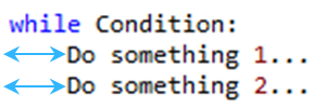
看起來好像跟if差不多,其實也沒錯,當condition是True的時候,就執行之下的dosomething,跟if一樣的是要有:號跟內縮(我還是做了記號),跟if不同的是,while loop下的程式碼,會一次一次的被執行,一直到condition變成False為止。喔,這句話好像很重要,condition到最後要變成False,才會停止。我們來試試看。
a = 1
while a < 10:
    print(f"a = {a}")
ㄟ嘿,這樣行了。歸納一下,如果我們想要程式執行固定次數,例如10次,那我們需要一個開始點(例如a =0),一個結束點(例如a<10),一個步幅(就是每一次前進的距離,例如a=a+1)。上例中,如果我們想要印出來的是1,3,5,7,9呢?那就把a+=1改成a+=2,也就是每跑一輪,就讓a的值增加2(步幅為2)。那若是想要印出2,4,6,8呢?那就讓a一開始等於2。那若是也想印出10呢?這更簡單了,讓condition變成a<=10即可。
接下來我們再試一個例子來計算1+2+3+…+100 = ?程式碼如下:
s = 0 #sum
a = 1
while a <= 100:
    s += a
    a += 1
print(f"sum = {s}")
記得我們需要的答案是相加之後的總和,所以設計一個變數s來記錄相加後的值。而變數a就是控制相加次數而且因為a剛好也等於1~100,所以每次都把a加到s上,最後得到的s就是總和了。我們把print()寫到while loop的外面,因為若是寫到裡面,也會跟著被印100次,當然如果你想看到每次加了新數後的結果,那就大膽的print()放進while loop內吧!只是會印出不少東西就是。
我們已經知道while後面的條件是一個boolean值,也就是說若是寫while True:這樣是合法的。在介紹if的時候,我們提到if True是多此一舉,因為無論有沒有寫,都會執行。但是while True的情況就不同了,這個情況會讓while之下的指令無止盡的執行下去,直到天荒地老,海枯石爛,電腦壞掉,或是沒電的時候才會停(當然你還是可以按Ctrl+C來強制中止),那我們可不可以這麼做呢?答案是肯定的,為什麼,因為我們有王牌剋星break,break這個關鍵字,就是用來中止loop使用的。例如:
while True:
    print("Execute instructions")
    break
嗯,嗯,感覺好像是對,又好像怪怪的。這跟使用if True:好像效果一樣,while不是可以做很多次嗎?這樣只會做一次不是?原來我們還是需要一個計數器,好比說我們想要印個5次吧,那就加上次數控制,如下:
i = 0
while True:
    if i >= 5:# or i==5
        break
    print("Execute instructions")
    i += 1
因為要使用break,所以使用if,在某特定的條件下停止。除了break之外,還有另一個相關的關鍵字是continue,這個關鍵字與break不同,break是中斷整個loop,而continue被執行後,在loop中continue後面的程式碼不執行,直接跳回到loop中的開端開始重新執行。例如:
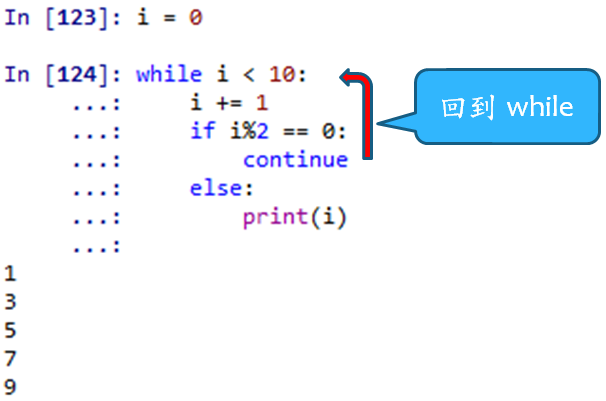
當執行continue後,程式便跳回到while開始重新執行。
-
Recap
- while loop語法介紹
- 如何處理無窮迴圈以及如何設計有限迴圈
- 關鍵字break與continue之介紹
第十五話、while loop (II)
現在大家應該對while loop的使用有深刻的認識了。事實上while loop的強大跟使用時機最主要就在於不確定使用次數的情況,咦,這好像跟之前提的有點不同,好吧,依照慣例,先來個例子說明。不過在此我們要先介紹一個函數input()。input()函數可以讓我們取得鍵盤輸入的值,這真是非常神奇,用一個簡單的函數來取得輸入值,現在先試試看:z = input() print(z)可以看出來,當我們輸入18後,18的值便被指派給z,要特別注意的一點是,傳進來的值是字串(str)。input()這個函數還可以在小括號內給一個字串參數,當作提示字元,這樣使用者可以明白需要我們輸入甚麼,例如:
age = input("請輸入你的年齡:\n")
print(age)
容易吧,不過年齡好像還是用整數(int)比較合理,沒問題,之前學過了,只要把它cast成整數就好了,使用int(age)即可。好了,學會這個做甚麼?現在設計一個簡單的小程式,它會印出來我們輸入的內容,一直到我們輸入quit為止。試試看。
while True:
    i = input("輸入quit來離開程式:\n")
    if i=="quit":
        break
    else:
        print(f"你輸入了\t{i}")
這個小小的程式很好的說明了while loop的強大,我們無法事先知道這個loop需要維持多久,執行多少次,它的停止條件是當輸入的內容為quit字串,因此只有quit出現後才會跳出。現在把之前計算BMI的程式拿來修改一下,讓我們可以自行輸入身高體重的數值,而且可以隨時輸入特定的內容來中斷它,如下(Talk15_1.py)。
while True:
    # 提示如何中斷程式
    print("隨時輸入quit來結束")
    # 取得身高
    weight = input("請輸入體重(kg):\n")
    # 判斷是否為quit
    if weight=='quit':
        break
    else:
        weight = float(weight)
    # 取得體重
    height = input("請輸入身高(cm):\n")
    # 判斷是否為quit
    if height=='quit':
        break
    else:
        height=float(height)/100.0

    # 計-bmi
    bmi = weight/height**2

    # 根據bmi判斷狀況
    if bmi < 18.5:
        print(f"你太瘦了,bmi={bmi}")
    elif bmi < 23.9:
        print(f"你是標準身材bmi={bmi}")
    elif bmi < 27.9:
        print(f"你要控制一下飲食了,bmi={bmi}")
    else:
        print(f"肥胖容易引起疾病喔",bmi={bmi}")
這個內容長一點,解釋一下。一開始先提示如何中斷程式,這是一個好習慣,不然使用者無法知道怎麼結束。接著跟之前一樣利用input()來取得輸入值,不過每次取得一個輸入值,都判斷一次是不是等於quit,如果等於就中斷(break),否則就繼續。在input()的提示字元內加上單位,這也是好習慣,讓使用者可以輸入正確的數值。通常我們身高習慣說幾公分,所以記得在計算bmi的時候要換算成公尺。剩下的就跟之前相同了,如果你都懂了,很棒,已經可以設計一個完整的程式了。
在Python的while loop語法中,設計了一個號稱不太成功的語法,就是跟else連用。也就是說,Python中可以使用以下語法:
while Condition:
    do something 1...
    do something 2...
else:
    do other thing 1...
    do other thing 2...
現在問題是,else之下的指令在甚麼情況下會執行?在if...else...中,很清楚else是在if為False的時候執行,那while…else…呢?我們先設計個例子試試看。
while a < 5:
    print("這是真的")
    a += 1
else:
    print("這是其他狀況")
唔,跑完了while後又跑了else,那這個else有寫跟沒寫不是一樣嗎?把上面的程式修改一下再試試看。
a = 1
while a < 5:
    if a == 3:
        break
    print("真的")
    a += 1
else:
    print("其他狀況")
咦,這次沒執行else的內容,兩個的差別是甚麼呢?原來是當while loop被break的條件下,便不會執行else的內容,也就是說else會在while順利執行完畢的情況下執行。那這有甚麼用?有些人建議不要用,Well,確實不用也能完成要做的事,不過如果能確實掌握意義,要也不失為一個手段,我們可以嘗試以下例子:
i = 0
r = int(input("輸入列印範圍:\n"))
while i < r:
    if i >= 10:
        break
    else:
        print(f"i = {i}")
        i += 1
else:
    print("i的值小於10")
當輸入的值為5,表示while loop不會中途被中斷,所以會執行else的指令,如果輸入的值大於10,那麼while loop會被中斷,所以不會執行else的指令。 【若要在console裡輸入多行指令,請按Ctrl+Enter】
-
Talk15_1.py
- 使用input()來設計鍵盤輸入
- while loop與break及else的連用
Recap
第十六話、for loop
之前一話介紹了while loop,它的含意是當某個情況存在時,程式會不停的執行,直到該情況消失為止,這個語法可以適用於不確定要執行幾次的狀況。一樣是loop,for loop的使用通常較好應用於確定要執行幾次的狀況。先看一下語法。for i in range(10): do something 1... do something 2...都是新單字,現在逐一來解釋。for是for each的簡寫,就是說對每一個。對每一個甚麼?後面接著i,就是說對每一個i,i是變數名稱,你可以給任意名字,通常習慣是用i是因為指稱index(索引)這個字。那麼i是?i是in range(),也就是在某範圍。整個說起來就是【對於在範圍內的每一個i】,冒號之下就是要做的事情。range()這個函數會產生一個範圍內的數列,舉個例子來說,如果range指的是1,2,3,那就是表示i=1, i=2, i=3三個輪迴,我們會做一些事(for loop之下的指令)。說了很多,不如舉個例子,看下例:
for i in range(5):
    print(i)
剛才說i對應的是range()所產生的數列,可見產生的數列是0,1,2,3,4,這真是太神奇了,傑克,之前我們使用while loop的時候,要達到執行5次這個效果,需要先設計一個變數(i),設計開始值(0),設計結束值(5),設計步幅(1),現在一句話i in range(5)完全搞定了。當我們給range()這個函數一個參數時(如上例的range(5)),代表的是預設開始值為0,預設步幅為1,而所給的數值原則上就是結束值,也剛好是要執行的次數。如果我們想要改變開始值要怎麼做呢?
for i in range(3, 10):
    print(i)
看起來直接給兩個參數即可,一個是開始值(3),一個是結束值(10),而其步幅預設為1。而且我們發現,i會等於開始值,卻不會等於結束值,也就是說i逐次等於開始值到結束值-1。此外,range()還能這樣使用。
for i in range(1, 10, 2): print(i)很顯然1為開始值,10為結束值,而2為步幅。事實上這個才是完整型態【range(起點,終點,步幅)】,前面兩個寫法只是省略了部分參數,直接使用預設值罷了。在Python中,步幅可以是負的,也就是每次都減少,例如:
for i in range(5, 0, -1):
    print(i)
這樣是不是很方便,當要執行的次數我們心裡有數的情況下,for loop比while loop來得更簡單直覺,倒不是while loop無法達到一樣的效果,不過for loop更優秀而已。接著用for loop來設計之前寫過的1+2+…+100這個程式,如下:
s = 0
for i in range(1, 101):
    s = s + i
print(s)
再次強調因為我們也要加上100,所以range上限要寫101,表示100會被包含。假設我們要執行的內容,跟i沒有關係,僅跟次數有關,也就是內容不會包含i,那還是可以使用i,不過有些人會建議既然如此,就使用個底線來代替變數,這樣我們就知道變數不會被使用,例如:
for _ in range(3):
    print("選我")
反正跟變數無關,只要確定次數即可。
for loop跟while loop除了語法有點差異,但目的完全相同,所以搭配的關鍵字也都相同,例如都可以使用break跟continue。
for i in range(10):
    if i%2 == 0:
        continue
    else:
        print(i)
    if i==7:
        break
也一樣可以跟else搭配(如果無法掌握是可以不用),在loop沒被中斷的情況下執行else。
for i in range(6):
    if i%2 == 0:
        continue
    else:
        print(i)
    if i==7:
        break
else:
    print("沒碰到7")
-
Recap
- 介紹for loop的語法
- 了解range()的用法
- for loop與break、continue、以及else的合用
第十七話、loop之老生常談
我想現在loop對各位來說算是小菜一碟了。接下來我們來設計一個程式印出九九乘法表吧。這要怎麼做呢?首先我們先想想1的情況,1x1=1, 1x2=2,…,嗯,乘數不動,被乘數每次+1,每次+1這個我們在行,先弄個1的試試看。for i in range(1,10): print(f"1x{i} = {1*i}")簡單。那麼若要把其他的2,3,…,9也都印出來呢?嗯,好像把上面的1換成1~9就好了,1~9聽起來是一個loop可以搞定的,那就把上面這個for loop放進另一個for loop內,有道理,試試看。
for j in range(1,10):
    for i in range(1,10):
        print(f"{j}x{i} = {j*i}")
有了,印出很長的九九乘法表,這裡就不顯示了。在for loop裡面有for loop稱之為巢狀結構(Nested),事實上我們之前已經用過很多巢狀結構了,例如if裡面有if,else裡面有if...else...,while裡面有if…else…。一個for loop執行9次,兩個相嵌的for loop就會執行9*9=81次。所以兩個for loop是一個二維的空間概念,我們先來嘗試以下的例子。
for i in range(10):
    print("*", end = "")
咦,這是做甚麼?之前我們使用print()的時候,印完就直接換行,那是因為裡面的參數end的值預設是換行("\n"),如果改為""表示不要換行。那這個loop就會印出一行10個*。如果我們要印10行這個,就是要把這個for loop執行10次,很明顯要把它放進另一個執行10次的for loop內,如下:
for j in range(10):
    for i in range(10):
        print("*", end = "")
    print()
記得在最外面的for loop每執行一次要做一次print()讓它換行。這樣的方式可以產生兩個維度的內容。那如果我們想要第一行1個*,之後依序每加一行就增加一個*,最後形成一個三角形,要怎麼做呢?
for j in range(1, 11):
    for i in range(j):
        print("*", end = "")
    print()
也可以變成倒三角形,如下:
for j in range(1, 11):
    for i in range(j, 11):
        print("*", end = "")
    print()
容易吧。不過其他語言這樣做是OK,但是Python卻可以有更簡便的方法,還記得之前提到字串乘以一個數字會發生甚麼事嗎?
for i in range(1, 11):
    print("*" * i)
嘿,這是特殊情況,對於了解巢狀結構沒有幫助。
這一話的最後來做一個比較複雜的例子,我們想要印出小於200的所有質數,要怎麼使用程式來完成呢?唔,質數啊,定義是指能被1跟自己整除的數,也就是只有兩個因數(1跟自己),特別注意最小的質數是2。那好吧,首先我們要能夠判斷一個數是不是質數,合理吧?
m = 9 # 要被檢測的數
isPrime = True # 先假定是質數
for i in range(2,m):
    if m%i == 0: # 表示不可能是質數了
        isPrime = False
        break
if isPrime:
    print(f"{m}是質數")
使用上面的程式碼,不用else的話,使用if…判斷isPrime是否為True,是True表示m是質數。若是使用else則如下:
m = 9 # 要被檢測的數
isPrime = True # 先假定是質數
for i in range(2,m):
    if m%i == 0: # 表示不可能是質數了
        isPrime = False
        break
else:
    print(f"{m}是質數")
接著要得到小於200的所有質數,那好,把上面的m變成2-200就行了。
for m in range(2, 200): # 要被檢測的數
    isPrime = True # 先假定質數
    for i in range(2,m):
        if m%i == 0: # 表示不可能質數了
            isPrime = False
            break
    else:
        print(f"{m}質數")
嗯,也不是那麼難,對吧。多練習才是王道,以下幾個小問題供各位玩耍:
1. 請問該如何找出小於某數n的自然數中,所有與n互質的數?互質的意思就是兩個數的最大公因數為1。
2. 如果一個數除去本身之外的所有因數和等於本身的話,我們將之定義為Perfect Number。例如6的因數為1,2,3,6,又符合1+2+3=6,所以6是Perfect Number,而1+2+4≠8,所以8不是Perfect Number。請問如何判斷一個數是否為Perfect Number?如何找出介於m跟n兩個數之間的所有Perfect Number?
3. 如果一個數的組成數字的三次方和等於該數,那麼該數稱之為Cube Number。例如 ,所以153稱之為Cube Number。請問該如何判斷一個數是否為Cube Number?請問要如何找出介於m及n之間所有的Cube Number?(可以先練習三位數字就好,即數字介於100到999)
- 1+2+3+4+5+...+N
- 12+22+32+...+N2
- 0+1+1+2+3+5+8+...+N
- 1+2+2+3+3+3+4+4+4+4+5+5+5+5+5+6+...+N
- 1+1/2+1/3+1/4+1/5+...+1/N
- 1-1/2+1/3-1/4+1/5-...+1/N
5. 請問該如何求得n!的值?(請注意0!=1!=1)又請問該如何求得1!+2!+3!+...+n!的和?
-
Recap
- 使用for loop設計程式列出九九乘法表、繪出三角星陣、以及求得質數
第十八話、函數
在寫程式的時候,經常會寫錯,可能心神不寧,可能人有錯手,這要怎麼避免呢?一個很好的方法就是一小塊一小塊地進行程式碼創作,最好每完成一小塊就測試一下,這樣錯誤發生就會減少。而如果這一小塊一小塊的程式是需要被重複使用的,那就更好了,正確的內容只要複製過來就好了。以上都是函數的好處,不過使用函數就不需要到處複製了,我們需要的是呼叫(call)它。現在先來看看函數怎麼建立?def functionName(): do something 1... do something 2...建立函數使用的關鍵字為def,在其後加上我們幫函數取的名字(要記得還是要符合之前提到的命名規則),然後加上小括號(),冒號(:)之後跟之前if,while,for類似,內縮表示函數內要做的事情。首先先來看一個最簡單的例子:
def fun1():
    print("一個小小函數")
fun1()
當我們輸入指令fun1(),記得要有小括號,表示我們呼叫了fun()這個函數,程式便會執行函數內定義的內容。記得我們剛剛說最好它可以重複使用嗎?現在我們來多呼叫幾次這個函數。
for i in range(5):
    fun1()
這樣好像沒看出太多效果,不過想像一下如果函數內定義的內容很長的時候,那就會節省很多時間跟打字了,畢竟只要建立一次,就可一直到處使用。
現在回想一下,之前我們已經多次提到函數並使用了,例如print(),type(),id(),input()等,果然都有小括號,,不過他們的小括號裡面好像都可以給參數,這個參數是為傳入參數(arguments),我們也可以設計看看。
def fun2(a):
    print(f"{a}的平方為{a**2}")
fun2(8)
很好,只要在呼叫的時候把需要輸入的內容寫在小括號內就好了。不過如果我們想要計算例如12+22+32+42+52=?可以使用這個函數嗎?難道要我們把平方值寫下來然後相加嗎?當然不是這樣,這個時候我們需要函數傳回來我們需要的值,然後我們再來做進一步的計算,想要函數傳回資訊,需要使用到關鍵字return。
def fun3(a):
    return a**2
print(fun3(3))
可以看出來fun3(a)這個函數,接受一個輸入值,並傳回該值的平方。所以當我們print()的時候,小括號內的是為該函數的傳回值。也就是說,fun3(3)就是9。那現在可以來求解上面的問題了。
fun3(1) + fun3(2) + fun3(3) + fun3(4) + fun3(5)嘿,我們好像做了一件蠢事,怎麼不用個loop搞定呢☻?你能看出這點,也能寫得出來,對吧。剛剛的例子所傳入的參數只有一個,應該可以傳入多個吧?那當然,只要使用逗號分開就好了。
def fun4(w, h):
    return w*h
fun4(10, 8)
好了,基本的函數設計現在會了,來把它用在之前的找出小於200的所有質數這個問題上。一樣的邏輯,我們只要寫一個函數,每次傳入一個數字,經過計算後,它必須傳回是否為質數,之後只要一直給它數字讓他判斷即可。
def isPrim(n):
    for i in range(2,n):
        if n%i == 0:
            return False
    else:
        return True

for i in range(2, 200):
    if isPrim(i):
        print(f"{i}為質數")
應該不難理解吧。
假設我們有兩個函數A跟B,A的內容是呼叫B,而B的內容是呼叫A,這樣會發生甚麼事?試試看。
def funA():
    print("Inside funA")
    funB()

def funB():
    print("Inside funB")
    funA()
好吧,如果你真的無聊到去執行funA(),你會發現這就好像是無窮迴圈,好像我們也沒有設計讓它停止的機制,這甚至比無窮迴圈更快的到達系統可以接受的上限而出現錯誤停止。不過我們可以將其稍作修改,給他們一個停止的機制,如下:
def funA(a):
    print(a)
    if a <= 0:
        return
    a -= 1
    funB(a)

def funB(a):
    print(a)
    if a <= 0:
        return
    a -= 1
    funA(a)
此時呼叫funA(10)的話,會出現10到0的數字,因為我們這次有停止機制(a<=0)了,特別強調一下return可以獨自使用,意思就是結束函數,但是沒有傳回甚麼。通常我們不會這樣呼叫其他函數來來回回多次,不過倒是會呼叫自己多次,這個留待後面討論。
順帶一提的是,在Python中的函數也是一種物件,所以也可以指派給某個參數,例如:
def square(x):
    return x**2
s = square
print(s(5))
當square被指派給參數s後,s便是函數square了。
-
Recap
- 建立一個函數(def)
- 設計函數的傳入參數以及傳回值
- 函數可以指派給變數
第十九話、keyword arguments
之前提到過函數可以給多個傳入參數,當我們在使用函數的時候,需要一個一個對應輸入,函數設計時設計了幾個傳入參數,呼叫時就要給幾個傳入,這樣的參數稱之為positional arguments。不過若是參數有初始值就不一樣了,若是有初始值,即使沒傳入也可以使用初始值,此稱之為keyword arguments。例如:def usToNt(dollars, rate = 30.141): print(f"You have ${dollars}, which equals to NT.{dollars*rate}") usToNt(100) usToNt(100, 31)可以看出來,如果只輸入一個參數,表示匯率(rate)使用初始值(30.141)。在設計函數時,有初始值的參數必須在沒有初始值的參數後面,所以我們不能夠設計如下函數:
def usToNt(rate = 30.141, dollars):
    print(f"You have ${dollars}, which equals to NT.{dollars*rate}")
這是為什麼呢?是因為如果這樣設計可以的話,那如果我們呼叫函數時只給一個傳入參數,程式無法判斷這個傳入的參數是要把值給rate還是dollars,所以在設計的時候,必須讓沒有初始值的在前面,而沒有初始值的參數是一定需要在呼叫的時候傳入值的。此外,在呼叫函數的時候,我們可以把原始設計的參數名稱加在輸入裡,這樣有時會更清楚。例如剛剛的函數,我們也可以這樣呼叫:
usToNt(100, rate = 30.5)
usToNt(dollars = 100, rate = 30.6)
usToNt(rate = 30.6, dollars = 100)
唯一不能使用的方式就是:
usToNt(rate = 30.5, 100)一樣的,不能把有初始值的keyword argument放在positional argument的前面。現在練習設計一個無腦的函數如下:
def fun(a = 1, b = 2, c = 3):
    print(f"{a},{b},{c}")
fun()
fun(7,8,9)
fun('a')
fun('a','b')
fun(b = 8, c = 9, a =7)
這些執行函數的方法都是正確的,只是我們要確定是對應到哪個變數。需要強調的是,不是keyword arguments才可以使用變數名稱來指定其值,根據之前的例子(usToNt),即使沒有初始值,還是可以使用變數名稱。例如:
def positional_fun(a,b,c):
    print(f"{a},{b},{c}")
positional_fun(a = "do", b = "re", c = "mi")
positional_fun(b = 8, c = 9, a = 7)
也就是說,如果我們知道原來定的變數名稱,那將值指派給該變數(e.g. a="do")這樣的方式是絕對不會錯的,即使它不是keyword arguments。
-
Recap
- 如何設計及使用keyword arguments
- 如何與positional arguments並用
第二十話、註解文字(docstring)
在建立函數的時候,我們應該適當的給予註解,事實上在程式的每個角落,都應該要適時的加入註解,之前我們已經提過可以使用#字號來加入單行註解,現在來介紹一下整段註解。整段註解因為是可以跨好幾行文字,所以在Python中使用多行字串(使用’’’’’’或””””””來包含的文字)來充當註解,所以在程式中,若是沒有將其指派為某變數,則為註解。例如:""" A function named func() Second line... """ def func(): print("func()")三撇所包含的內容是為註解。有時候我們常會為了測試,要先讓某一部份的內容不執行,有時恢復執行,我們可以使用註解來切換,因為變成註解的內容便不會執行,我們可以這樣做。
#"""
#A function named func()
#Second line...

def func():
    print("func()")

#"""
最上面的#字號去除後,整個函數就變成註解,加上後就可以執行,方便吧。在Python中,函數的第一行如果是註解,那就可以在help的時候顯示,這個註解文字可以幫助我們了解函數,且可以快速查詢到函數的意義,所以我們應該這樣做。
#'''
def func():
    """
    A function named func()
    This is the second line...
    """
    print("func()")
#'''
Run了之後,若在console內打help(func)指令來查詢func()這個函數,可以看到我們剛剛寫的註解變成解釋函數內容的文字,只要使用help來查詢即可。
help(func)註解文字名為docstring,也是因為它被儲存在funName.__doc__這個變數內的關係。
要特別注意的是必須是在函數內指令的第一行之註解才會變成docstring,例如若是在print()後面的註解便不是docstring,而且只能是第一個註解,也就是說如果函數內容一開始就定義兩個註解,那麼僅有第一個會變成docstring。此外,即使是第一行,若是使用#字號的註解,也不是docstring。測試了一下,使用""形成的註解文字也可以當作docstring,不過""只能使用於單行。以下為正式的例子。
def theBigger(a, b):
    """
    比較a,b兩數並傳回較大者
    若兩數相等則傳回任一數
    """
    if a > b:
        return a
    else:
        return b

print(theBigger.__doc__)
help(theBigger)
再測試一下如果不只一個註解的情況。
def theBigger(a, b):
    """這行變成第一行"""
    """
    比較a,b兩數並傳回較大者
    若兩數相等則傳回任一數
    """
    if a > b:
        return a
    else:
        return b

help(theBigger)
此時的函數說明變成第一行,也就是說第一個註解才會成為docstring。我們應該盡量針對每一個函數都設計docstring,如此較好查詢理解函數內涵也可增加程式的操作性。
-
Recap
- 程式內的註解文字(#、”””、’’’)
- 函數的註解以及使用help()查看函數的註解
第二十一話、lambda
lambda這個關鍵字,指的就是函數,也有人稱之為匿名函數,也就是說設計這個函數不需給函數名,而且比較簡短。來看一下下面例子。s1 = lambda x: x**2 s1(5)lambda這個關鍵字就是函數,:號之前的就是傳入參數,:號之後的就是傳回值。簡單吧,原則上就是以下這個函數的縮寫。
def square(x):
    return x**2
s2 = square
print(s2(5))
一般來說,lambda常用在其他語法內需要一個簡短函數的情況,甚至當作函數的傳回值(也就是說一個函數傳回值是一個函數,神奇吧)。
def aFunc(n):
    return lambda x: x%n
f = aFunc(3)
print(f(10))
首先aFunc(3)表示n=3,傳回一個函數給f。f(10)表示x=10,此時可計算10%3的值。其實也可以像下面的寫法。
ff = aFunc
print(ff(3)(10))
ff(3)就是呼叫函數aFunc(3)的傳回值,而此傳回值又是一個函數,這個函數接受一個傳入參數,所以後面加上(10)。
-
Recap
- lambda函數的介紹
- 函數可以是函數的傳回值
第二十二話、區域變數與全域變數
變數依其定義的位置不同,可分為區域變數(local variable)與全域變數(global variable)。這兩者的差別是甚麼?主要是區域變數只能在特定區域被使用。先看一下下面的例子。def afunc(x): x = 5 print(f"x = {x}") afunc(1) print(f"我也來印{x}")如果執行上面的程式,會出現錯誤(NameError: name 'x' is not defined),這是因為x僅在函數內能被使用,不能在函數外要使用它,所以程式傳回錯誤。所以若是在函數外面定義的話,就會變成全域變數,那就能被使用了。例如:
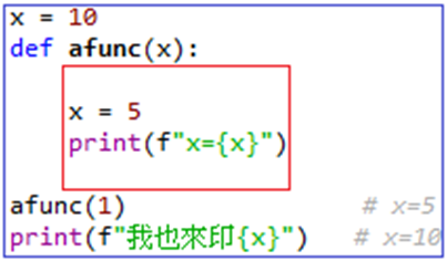
現在可以正常執行了,而且函數印出x=1,而函數外print()取得x=10。也就是說,函數內為區域變數,可使用範圍為紅色區域,而函數外自x=10宣告後,藍色區塊為全域變數的可使用範圍。要注意的是在函數內的x=5,改變的是區域變數的值,而不是全域變數的值。其實若是要做指定運算,在函數內即使是全域變數也無法被使用。將上面的程式修改如下。
x = 10
def afunc():
    x = x + 1
    print(f"x = {x}")

afunc()
print(f"我也來印{x}")
雖然有全域變數x,但是在函數內還是不允許對x做指定運算,所以會出現錯誤。在這情況下如果想要取得x來做運算,第一當然可以使用其他變數名(e.g. k=x+1,然後印k),此外也可以使用關鍵字global來得到全域變數。
x = 10
def afunc():
    global x
    x = x + 1
    print(f"x = {x}")

afunc()
print(f"也來印{x}")
global x的意思就是跟程式說現在要用的是全域的x。
在lambda那一話中提到回傳值可以是函數,所以可想見函數內可以包含其他函數,那其中的變數作用區域又是如何?先看以下例子:
執行程式看看結果為何。嗯,符合我們的期待,每個變數x的影響範圍與其被定義的位置相關。那麼如果把bfunc()內的x設為global,會取得那一個x的值呢?是往上一層,還是最外面?試試看。
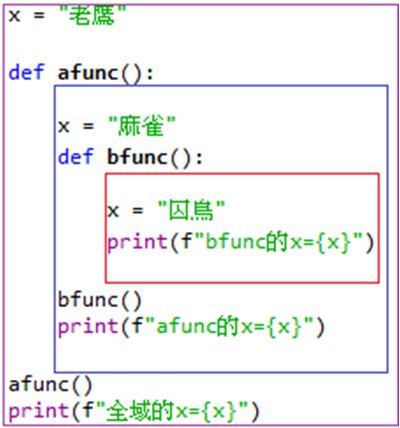
x = "老鷹"
def afunc():
    x = "麻雀"
    def bfunc():
        global x
        x = "囚鳥"
        print(f"bfunc的x = {x}") # 囚鳥
    bfunc()
    print(f"afunc的x = {x}") # 麻雀
afunc()
print(f"全域的x = {x}") # 囚鳥
結果如註解。可見使用global是直接取得最外面的global variable,不愧global這個名字。那有沒有辦法抓到上一層的變數?Python設計另一個關鍵字nonlocal,可以讓我們取得上一層的變數,做法如下:
x = "老鷹"
def afunc():
    x = "麻雀"
    def bfunc():
        nonlocal x
        x = "囚鳥"
        print(f"bfunc的x = {x}") # 囚鳥
    bfunc()
    print(f"afunc的x = {x}") # 囚鳥
afunc()
print(f"全域的x = {x}") # 老鷹
afunc()內的變數被修改了,因為nonlocal讓bfunc()內的x變成上一層的x。不過要記得不能將afunc()內的x定義為nonlocal,因為外面的變數是global。最後再看一下下面的例子。
x = "老鷹"
def afunc():
    x = "麻雀"
    def bfunc():
        print(f"bfunc的x = {x}")
    return bfunc()
afunc() # 麻雀
print(f"全域的x = {x}") # 老鷹
這個例子中,bfunc()是afunc()的傳回值,當呼叫afunc()後,得到的應該是一個函數(也就是bfunc),而這個函數中的變數卻保持著傳回時的變數值,這稱之為closure。即使x變數不是定義在bfunc()內,而傳回值應該只有包含函數,但bfunc()再被傳回時,還是保存著x的內容,也就是說closure會傳回函數的整個執行環境。
-
Recap
- 區域變數與全域變數的區別
- global與nonlocal關鍵字的使用
- 了解closure
Python亂談
資料結構
第二十三話、List
List是一種資料結構,就是讓我們裝資料的地方,或說是一種容器(container)。這是Python內建的container。如果要設計的程式會牽扯到一堆的資訊,那麼我們就得考慮怎麼編排這些資訊,希望這個編排的方式可以方便我們工作,而list就是其中的一種。list是形狀是一串的資訊,每一筆資料有一個索引值(index),我們可以根據索引值來取得資料內容。舉例說明: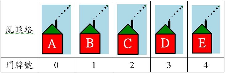
假設亂談路有五戶人家(A,B,C,D,E),門牌號碼分別為0,1,2,3,4,我們可以得到亂談路2號是住C小姐。list就類似是這一條路,每一個空格中住著一戶人家,每一個空格也都有一個index(門牌號),所以我們也可以根據索引值很容易地得到list內儲存的物件。那要如何建立一個list呢?先看一下help。
help(list)根據其定義,建立list可以使用以下方法:
- 使用list函數,例如alist=list()來建立一個空的list
- 使用list函數,傳入參數為一個iterable,則可根據iterable產生list
解釋一下何謂iterable的物件,定義是一種可以逐一取得內容的物件,例如之前學過的range(),或是目前正在學的list。在Python中,這樣的物件會包含一個名為__iter__的方法,可以讓我們得到一個iterator,而iterator物件會包含__next__方法,next可以讓我們逐一得到下一個內容,直到走遍所有內容。
因為list是重要的內建容器,所以除了上面兩個方式之外,還提供了另一個簡單的方法如下:- 直接使用中括號,例如blist=[]
alist = list()
print(alist)
blist = []
print(blist)
clist = list([])
print(clist)
以上形式都可以,要注意的是上面的例子建立的都是空的list,裡面沒有包含任何物件。若是在一開始想要給初始值,可以使用如下方式:
blist = list([1,2,3,4,5])
print(blist)
clist = [1,2,3,4,5]
print(clist)
list的內容可以是隨意的物品,並不一定需要是相同型態,所以也可以建立如下的list。
alist = [1, "2", True, 3.14159, ["do", "re", "mi", 7, 8, 9]]
print(alist)
當然通常為了方便操作,大部分都會在同一個list內放置相同類型的物品,除非我們可以確定每一個位置放置哪種類型的物品。
-
Recap
- list 的介紹以及如何宣告
- iterable就是元素可以被逐個拜訪的物件
第二十四話、List的存取
在前一話中介紹了如何建立list,接下來介紹如何操作list。首先先看如何存取list內的物品。之前我們介紹了亂談路2號是C小姐,而取得list物品的方式也一樣。例如:lista = list(range(1,20,2)) print(lista) print(lista[5])在此我們建立了一個list名為lista(路名),其中索引值(門牌號碼)為5號的物品為11,再次強調list的索引值是從0開始,假定list的長度為n,則最後一個物品的索引值是n-1。我們可以使用len()這個函數得到list的長度(物件個數)。例如:
len(lista)因為lista的長度為10,所以可見索引值為0-9(包含9)。當我們不確定list總長度但想取得最後一個物品時,可以使用如下方式:
lista[len(lista)-1]先取得總長度然後減1,再利用這個數值來得到最後一個位置的物品。不過Python提供另一個更容易的做法如下。
lista[-1]
lista[-2]
索引值為-1表示後面算來第一個(也就是最後一個),-2表示後面算來第二個。不過要記得不能嘗試取得超過list範圍的物品,會出現錯誤,不過超過範圍便沒有物品了,那出現錯誤也是自然而然,不是嗎?
lista[len(lista)]不過要小心,
lista[-len(lista)]是正確的,表示第一個物品,這是為何,因為逆行方法的計算是從-1開始,而不是從0開始。
既然我們知道最小到最大的索引值,那麼若是要得到list內的所有物品,那麼使用個loop似乎是理所當然的事情了。
for i in range(len(lista)):
    print(f"lista[{i}] = {lista[i]}")
因為list本身是iterable物品,而for loop可以直接逐一取得iterable內物品,例如range(),所以我們也可以這樣寫。
for i in lista:
    print(i)
這樣簡潔多了。不過這樣好像又看不到索引值了。如果還是想要索引值,有另一個關鍵字可使用,稱為enumerate,它的意思就是協助我們列舉(自然是從0開始)。
for k, i in enumerate(lista):
    print(f"lista[{k}] = {i}")
這個例子中有兩個變數,i還是指的lista內的物品,而k則表示索引值(或說從0開始,每次增加1來列舉iterable的元素)。這是一個很好用的指令,應該多熟悉它。
在上面的說明中,不是得到一個,就是得到全部,如果我們想得到其中的一部分,例如第3個到第6個,那怎麼辦?原則上for loop還是可以幫我們搞定。例如:
start = 3
stop = 6
for i in range(start, stop):
    print(f"lista[{i}] = {lista[i]}")
這樣當然是可以的,不過Python提供我們便利的方法稱為切片(slicing),可以將一個list內的內容像切生魚片一樣的取出來,不過要注意的是切片出來的物件是另一個list。例如:
lista[3:6]喔,這真是太便利了,直接說3:6(index 3到6,根據Python的慣例,6不包含)就可以了。跟range()的數字產生類似,我們也可以每隔幾個取一次,只要給間隔(步幅)即可,例如:
lista[2:8:2]白話解釋就是從2開始,每隔兩個取一次,直到8為止(8不包含)。此外,開始或結束如果不給值,那麼就是從頭(0)或是到尾(len(lista)-1)的意思。
lista[:8:2]
lista[3::2]
lista[3:]
lista[:8]
lista[::3]
lista[:]
這些都是對的。若是要更改list內物品的值,則跟取得類似,將一個新的值指派給取得的值即可。例如:
lista[0] = 100很容易吧。事實上這個list就好像我們定義了10個變數,只是變數名稱稱為lista[0], lista[1], lista[2],…,lista[9]。
-
Recap
- 存取list中的元素,索引值為-1表示最後一個元素
- 使用切片(slicing)來取得部分list
- 使用enumerate()函數
第二十五話、List的新增元素
List的長度是可變動的,也就是說我們隨時可以增加或減少其中的元素個數。首先,如果我們有兩個list,那直接使用+號相加即可。例如:list1 = list(range(3)) print(list1) list1 + [3]記住使用+號僅可用於兩個list的情況。有+是不是就有-呢?事實上是沒有,不能使用一個list減去另一個list。那是不是有乘或除嘞?答案是可以用乘的,不過不是乘以另一個list,而是乘以一個整數,如下:
list1 * 3結果就是把內容重複幾次。
剛才說將兩個list使用+號連結,就可以把他們的內容相加到一個list內。不過這樣做的話,必須先分別拆開然後內容相加再合併成一個list,做的工作比較多,若是我們想要直接在一個list的後面附加一個元素,可以使用append()方法,例如:
list1.append(3)
print(list1)
要注意的是append是把傳入參數附加到list內使其成為最後一個元素,所以如果傳入參數是另一個list,那麼這個list將會成為元素,跟相加的結果不同。
list1.append([7,8,9])
print(list1)
[7,8,9]變成了最後一個元素,而不是打散成為list裡面的後面三個元素。如果要使用append來實現將兩個list內容相加,可以如此做。
list2 = list(range(3))
anotherList = [7,8,9]
for i in anotherList:
    list2.append(i)
print(list2)
不過如果是要達到這樣的效果,看起來還是使用list2+anotherList比較快。事實上除了使用+號外,Python的list確實有提供另一個方法來達到這個相加的目的,就是使用extend()這個方法。如下:
list2.extend(['a','b'])
print(list2)
這次加入一個字串的list,此方法的效果與list2+[‘a’,’b’]相同。上述的方法都是將物品加到list的最後,那如果我想加入到其他位置呢?這個情況使用的方法為insert()。
list2.insert(0,100)
print(list2)
list2.insert(2, ["new","in","town"])
print(list2)
傳入兩個參數到insert(),第一個是要加入的位置,第二個是要加入的物品,如此可以在任何位置插入物件。
-
Recap
- 使用+及*來合併或複製list
- 使用append()、extend()、insert()來加入元素
第二十六話、List的刪除元素
好了,學會了增加,再來學刪除。如果是要刪除某位置的物品,那麼使用pop()方法,例如:print(list2) list2.pop(2) print(list2)嗯哼,只要給位置(index)就能刪除了,要注意的是pop()這個方法傳回了被刪除了物件。如果不給位置,也就是沒有傳入參數的話,pop()會直接刪除最後一個元素。
list2.pop()
print(list2)
除了使用pop(),也可以使用del()來刪除(delete)元素,不同處是它的傳入參數為list索引值代表的元素。有點難解釋,看個例子就明白。
del(list2[0])
print(list2)
del並不是list的方法,所以不是使用list2.del()這樣的語法。本來list2[0]代表的就是元素100,但是也不能使用del(100),因為這樣看不來是要刪除那一個list,所以很自然地要用到del(list2[0])這樣的語法。而此方法的傳入參數可以是切片,這也表示可以一次刪除多個元素,舉例如下:
del(list2[3:5])
print(list2)
另一個情況是如果我們想要刪除一個list中的元素,但是我們不知道它的位置,那怎麼辦?假設我們有以下的一個list,
list3 = [1,2,3,3,4,5,5,6,7]假設我們想要刪除裡面的3,注意這裡面有兩個3,我們只要刪除第一個,若是我們不確定3的位置,那怎麼辦?可以這樣做。
for i in range(len(list3)):
    if list3[i] == 3:
        list3.pop(i)
        break
print(list3)
當然也可以利用enumerate來操作,請自己試試看。而Python中依然提供了一個方法來達到此效果,此方法為remove()。試著用這個方法來刪除list3中的5。
list3.remove(5)
print(list3)
Easy!不過如果我們的傳入參數並不包含在list內,會發生甚麼事?
list3.remove(10)出現了錯誤。如果我們想避免出現這個錯誤,那麼完整的刪除法變成要先確認這個物品是否在這個list內,如果有再刪除,嗯,聽起來很合理的邏輯,這裡使用關鍵字in來判斷list是否包含想要刪除的物品,如下:
if 10 in list3:
    list3.remove(10)
else:
    print("list3 does not contain 10")
好吧,最後來看一下如何刪除list的所有內容,事實上根據上面所學我們好像可以有好幾種方法,我們來嘗試看看並比較一下。
- 使用pop
list3 = [1,2,3,4,5,6,7]
for i in range(len(list3)):
    list3.pop()
print(list3)
還可以,每次刪掉最後一個。 - 使用del
list4 = [1,2,3,4,5,6,7]
del(list4[:])
print(list4)
這個好,直接刪除整個的切片。 - 使用remove
list5 = [1,2,3,4,5,6,7]
for i in range(len(list5)):
    list5.remove(list5[0])
print(list5)
每次都抓出第一個元素來刪除。
list6 = [1,2,3,4,5,6,7]
list6.clear()
print(list6)
如果只是為達目的的話,還可以這樣做:
list7 = [1,2,3,4,5,6,7]
list7 = []
print(list7)
讓list7直接指位到一個空list的記憶體,之前的留在記憶體,若沒再被使用,之後程式會自動回收(Garbage Collection)。最後提一下,若是整個list都不要了,則可以直接使用del來刪除。
list8 = [1,2,3,4,5,6,7]
del(list8)
print(list8)
此時不是list內容為空,而是整個list(變數)都被刪除了。
-
Recap
- 刪除list中元素,使用pop()、del()、remove()、clear()
- 使用in來判斷list是否包含某元素,使用del(list)來刪除整個list
第二十七話、List的刪除閒話
之前已經學會了如何刪除list內的元素了,可以使用pop、del、remove、clear等,在介紹remove的時候,說是可以刪除第一個出現(first occurrence)的符合元素,而我們感興趣的是如果想要刪除最後一個符合的元素,那要怎麼做?直覺的想法就是找到符合元素最後出現的位置,然後刪除掉,所以應該這樣做(為了方便重複操作,這裡寫成函數形式):li = [1,2,3,3,4,5,1,3,5,2,4] def removeLast(alist, element): p = 0 for k, i in enumerate(alist): if i == element: p = k # recoding the index of element li.pop(p) return alist print(f"{removeLast(li, 3)}")跑出來的結果確實是刪除了最後一個3。不過雖說名字叫做removeLast(),不過卻沒用到remove()方法。remove()這個方法僅能移除第一個出現的物品,若是可以將list倒過來就好了,還剛好有這個功能,稱之為reverse(),我們先看一下這個方法的使用。
li_1 = [0,1,2,3,4]
li_1.reverse()
print(li_1)
我們查看一下這個方法的help,可以看一下它的解釋。
help(li_1.reverse)最後特別的強調了*IN PLACE*,這是甚麼意思?in place的意思其實就是當我們呼叫這個函數後,它將list就地倒轉了,也就是說不可以寫li_1=li_1.reverse()。好了,既然list可以倒轉,那事情就簡單了,我們來建立另一個函數如下:
li = [1,2,3,3,4,5,1,3,5,2,4]
def removeLast2(alist, element):
    alist.reverse()
    if element in alist:
        alist.remove(element)
    else:
        print(f"{element} is not in {alist}")
    alist.reverse()
removeLast2(li, 3)
print(li)
只要倒轉過來刪除第一個然後再倒轉回來就可以了。
另一個問題是如果我們想要刪除li裡面最大的元素,那要怎麼做?先找到最大的位置然後再刪除它?聽起來很合理,我們試試看。不過因為最大的元素也可能不只一個,先假設我們要刪除的是list中第一個出現的元素。
li = [1,2,3,3,4,5,1,3,5,2,4]
def removeMax(alist):
    m = -99999
    for i in alist:
        if i > m:
            m = i
    alist.remove(m)
    return alist
removeMax(li)
print(li)
原則上removeMax()內大部分的程式碼都只是在找最大的值是哪一個?事實上Python的內建函數就有直接找最大(或最小)的函數了,是為max(或min)。所以如果有函數可直接找到最大的值,就可以直接刪除了。做法如下:
li = [1,2,3,3,4,5,1,3,5,2,4]
m = max(li)
li.remove(m)
print(li)
如果不在乎最後list內的物品排列順序,想要刪除最大的元素,也可以先將list內的元素按照大小順序排列後,直接刪除頭(或尾,端看是由小到大排還是由大到小排)即可。list內的排序方法為sort(),先試試看這個方法。
li = [1,2,3,3,4,5,1,3,5,2,4]
li.sort()
print(li)
li.sort(reverse=True)
print(li)
如果傳入參數reverse=True的話,表示由大到小排列。因為我們的目的是刪除一個5,所以使用由小到大排列,然後呼叫pop()即可。不過這樣的作法比之之前的方法來得費工,那是因為排序的演算是比較複雜的,用來做這件事有點像大砲打小鳥,不過因為list內容不多,又有現成的函數可用,差別就少了。
此外,如果不是要僅刪除掉一個5,而是要把所有的5都刪除的話,你應該知道怎麼做,對吧☻。
-
Recap
- 如何建立函數來刪除list中最後一個符合的元素及最大的元素
- 使用reverse()及sort()方法
第二十八話、多維list
說老實話,多維的list沒有甚麼太多可以說的,因為例如二維的list,只不過是一個list其中包含的物件都是一維的list。通常提到維度(dimension)或是自由度(degree of freedom),簡單的物理定義就是要描述它所需要的變數量。當我們想要得到一維list內的物品,僅需要一個變數(索引值)即能正確的得到,顧名思義,二維的list則需要兩個索引值,先來看一下二維list的例子。list2 = [[1,2,3],[4,5,6],[7,8,9]] print(list2) print(list2[1][2])list2中的元素都是一維list,所以我們要得到其中元素6的話,要先得到包含它的list,也就是list2[1],因為list2[1]也是一個list,所以要得到其中元素的話,要再次給定其在list的位置,所以是list2[1][2],需要兩個變數來指位。整個list2的顯示應該長這樣:
[[1,2,3],
 [4,5,6],
 [7,8,9]]
原則上2D的排列給行跟列的值來得到內容應該是很直覺的。若是要將裡面的元素一一萃取出來,那要怎麼做?1D的list我們知道用一個loop可以完成,2D的情況使用兩個loop應該算是合理。
list2 = [[1,2,3],[4,5,6],[7,8,9]]
for i in range(len(list2)):
    for j in range(len(list2[i])):
        print(f"list2[{i}][{j}] = {list2[i][j]}")
如果我們想要將list2內的元素都取出來,變成一個1D的list,那要怎麼做?原則上跟上述的做法差不多,只要能將內容一一取出即可,如下:
list2 = [[1,2,3],[4,5,6],[7,8,9]]
newList = []
for i in range(len(list2)):
    for j in range(len(list2[i])):
        newList.appen(list2[i][j]})
print(f"newList = {newList}")
若是3D的情形便是list內的元素為2D-list,若要走訪(traverse)最內裡所有元素,可以想見3D的情況是需要3個loop。你可以自己試試看。雖說沒甚麼可說的不過也說了一些,2D的陣列其實就是矩陣,所以在很多地方需要應用,Python有相關套件(Numpy)可以讓我們更好操作矩陣,將在之後提及。
-
Recap
- 如何建立多維的list
- 如何取得多維list內元素
- 如何使用for loop取出多維list內元素
第二十九話、list comprehesions
假設有一個list為clist = [1,1,2,3,5,8,13],我們想要得到一個新的list,內容是每個元素都是clist內的元素的平方,也就是[1, 1, 4, 9, 25, 64, 169],那要怎麼做?當然我們現在處理這個算是小小問題,簡單的一個loop可以搞定,如下:clist = [1,1,2,3,5,8,13] for k, v in enumerate(clist): clist[k] = v**2 print(clist)這樣做當然是對的,不過如果想要更Pythonic的話,可以使用list comprehesions。那麼何謂list comprehesions?其形式如下:
[expression for var in list[for...|if...]]這個形式會回傳一個list。在我們從小就學的數學中,曾經學過類似如下的符號表示:
{x2|x ∈ f(x)}
list comprehesions跟這個表示類似,只是把中間的直線(|)去除罷了。來看個例子先熟悉一下:
clist = [1,1,2,3,5,8,13]
[x**2 for x in clist]
第一個x**2表示要加進list內的值為x平方,後面是一個for loop來指出那些是x。這大概是Python獨有的寫法吧(也許其他語言也有,不過我孤陋寡聞沒看過),這樣的寫法可以讓程式碼更加簡潔,應該要多練習並多使用。現在再加上if...的條件進去,直接加在loop後面即可。
[x**2 for x in clist if x < 5]僅在x<5的條件下才進行。如果是for loop後面加上for loop的情況呢?
a = [1,2,3]
b = ['a','b','c']
[[x,y] for x in a for y in b]
原則上就是把兩個for loop套在一起,所以會出現所有的元素組合。如果是有3個list要顯示出所有組合,顯然可以使用3個for loop。
練習一個例子,使用list comprehensions來求得2到20的質數。
[x for x in range(2,20) if 0 not in [x%y for y in range(2,x)]]後面的list comprehensions每次會產生一個包含所有x%y的list,只要沒有包含0,則代表x為質數。我們也可以使用Python的內建函數all(),all的意思類似and,and需要兩個boolean都是True來傳回True,而all則需要整個list內的所有boolean都是True來傳回True。例如:
all([True, True, True, True, True])
all([True, True, False, True, True])
利用這個函數重寫剛剛的list comprehensions,如下:
[x for x in range(2,20) if all([x%y for y in range(2,x)])]
[x for x in range(2,20) if all(x%y for y in range(2,x))]
因為已經在list內,而且list comprehensions會回傳一個list,所以all()內的list comprehensions有沒有使用[]都可以。
也可以使用這個寫法:
[x for x in range(2,20) if not any(x%y==0 for y in range(2,x))]相對於all(),any()傳回True的條件便是只要list內有一個boolean為True。
-
Recap
- 如何使用list comprehensions來建立一個list
- 使用list comprehensions來建立一個包含質數的list
第三十話、傳值與傳址
當我們使用等號(=)後,左邊的變數值跟右邊相同了,例如:a = 10 b = a print(b) id(a) id(b) a is b其實a與b連編號都相同,表示兩者指向同一塊記憶體。但是無所謂,至少當我們改變b的時候,它就會指向另一塊記憶體。
b = b + 1
print(b)
id(b)
a is b
但是這樣的操作在其他物件例如list卻不一樣,例如:
lista = [1,2,3,4,5]
listb = lista
print(listb)
listb[0] = 100
print(listb)
print(lista)
id(listb)
id(lista)
搞了半天listb跟lista還是指向相同的記憶區塊,這稱之為傳址,也就是說等號只是讓另一個變數指向跟他相同的記憶體,這對於我們想要有一個獨立於lista之listb來說就不對了。換個方式做做看,
listb = lista[:]
listb[0] = 200
print(lista)
print(listb)
唔,分開了。其實這不算好方法,我們可以藉用list的copy()方法,如下:
listc = lista.copy()
print(lista)
listc[-1] = 500
print(listc)
print(lista)
再看下一個例子:
listx = [[1,2,3],[4,5,6],[7,8,9]]
listy = listx.copy()
id(listy)
id(listx)
listx[0][0] = 100
print(listx)
print(listy)
咦,不是已經copy了嗎?id也不同了,怎麼listy還是跟著listx變動?原來當結構裡面又有結構的時候,copy又不夠力了,沒有辦法一層一層的copy進去。那怎麼辦?自己一層一層的copy?好像可以。
listy = []
for i in listx:
    listy.append(i.copy())
print(listx)
print(listy)
listx[0][0] = 200
print(listx)
print(listy)
這樣可以了。不過如果裡面又有一層呢?或是超過一層呢?還好Python已經提供我們解答,做法如下:
from copy import deepcopy
listm = [[[1,2],[3,4],[5,6]],[[7,8],[9,10],[11,12]],[13,14,15]]
listn = deepcopy(listm)
print(listn)
listm[0][0][0] = 100
print(listm)
print(listn)
欲使用deepcopy這個方法,必須要先加上from copy import deepcopy這行指令來將此方法導入,import的用法在後面介紹,在這裡僅需記住要有這行指令才能使用即可。使用此方法,無論幾層內容都可以幫忙複製,在傳址的過程中,如果想要複製一個變數,要記得使用,免得最後結果出錯。
-
Recap
- List指派給另一個變數是傳址,可使用list.copy()來複製一個list
- 若是多層結構,可使用deepcopy來複製,需先import才能使用
第三十一話、未定長度參數函數
說著說著又回頭來聊函數了。這一話介紹未定長度參數(variable number of arguments)函數,意思就是說參數長度不確定,這是甚麼意思呢?看一下這個例子,如果我們想要知道某三個數的平均,那我們可以設計一個有三個傳入參數的函數,如果是想知道某四個數的平均,那要再設計一個有四的傳入參數的函數。都是算總和,但是卻因為參數數目不同而需要另外設計,能不能設計一個函數就好了?因應這個需要,Python提供我們設計變動數目參數的函數,先舉例如下:def varAve(*n): s = 0 for i in n: s = s + i return s/len(n) print(varAve(1,2,3,4,5))n前面加了個星號表示不確定會給幾個參數。其實你大概可以看出來了,這個*n不就是個list?當我們給了任意數量的參數,程式把這些參數都先放到一個list內來供我們使用。也就是說其實我們不這樣設計的話也可以直接讓輸入參數為list即可。順帶一提的是,若要加總一個list,可以直接使用Python的內建函數sum()來達成即可。
def varAve(*n):
    return sum(n)/len(n)
print(varAve(1,2,3,8,9))
之前我們提過函數的參數有positional arguments,也有keyword arguments,現在再加上不定數量的arguments,那在設計的時候要怎麼做?首先我們知道postional要在keyword之前,而未定數量的話很直覺的應該要放在後面,因為如果放在前面,我們將無法知道哪一個傳入參數將作為positional arguments。舉例如下:
def avescore(name, classNumber = 101, *score):
    ave = sum(score)/len(score)
    print(f"Average score of {name} in class {classNumber} is {ave}")
avescore("Tom", 102, 88, 92, 87)
這樣使用沒有問題,不過classNumber是keyword arguments,本來若不輸入是可以使用內定值的,可是在這裡若是不輸入的話,反而會出現問題(第一個分數會被當成班級別)。那把它放在最後如何?
def avescore(name, *score, classNumber = 101):
    ave = sum(score)/len(score)
    print(f"Average score of {name} in class {classNumber} is {ave}")
avescore("Tom", 88, 92, 87)
avescore("Tom", 88, 92, 87, classNumber = 102)
這樣倒是可以,不過要修改班級別,需要使用關鍵字classNumber。順帶一提,不能在一個函數使用兩個未定長度參數。如果有這樣的輸入要求,可以使用list。例如:
def avescore(name, *score, classNumber = 101, quiz):
    ave = sum(score)/len(score)
    ave2 = sum(quiz)/len(quiz)
    print(f"{name} in class {classNumber} has {ave} in exams and {ave2} in quiz")
avescore("Tom", 88, 92, 87, classNumber = 102, quiz = [69, 87, 91])
-
Recap
- 如何設計不定長度參數的函數
- 不定長度參數該如何與positional arguments跟keyword arguments合用
第三十二話、Function anotations
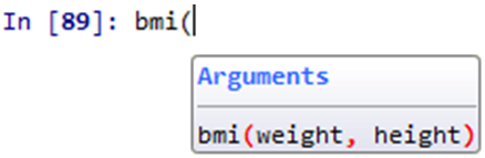
首先來看個我們知之甚稔的例子。def bmi(weight, height): """ Calculate Body Mass Index weight in kg, height in m return -> [bmi, Description] """ bmi = weight/height**2 # 根據bmi判斷狀況 if bmi < 18.5: return [bmi, "你太瘦了"] elif bmi < 23.9: return [bmi, "你是標準身材"] elif bmi < 27.9: return [bmi, "你要控制一下飲食了"] else: return [bmi, "肥胖容易引起疾病喔""] b = bmi(45, 1.65) print(f"Your BMI is {b[0]}, {b[1]}")在這個函數中,我們需要輸入兩個實數,會回傳一個list。當我們一開始碰到函數時,可以使用help()來先瞭解他如何使用。
help(bmi)當我們在使用函數的時候,也會出現提示。
不過在浩瀚的函數海中,總有我們不熟的函數,即使出現提示字元,也不確定要輸入甚麼內容,雖然可以使用help()來查看,但是如果在提示的時候給更多資訊就好了。因此,在Python 3提供了我們可以給函數參數註解的功能。我們再重寫上面的例子。
def bmi(weight:float, height:float)->list:
    """
    Calculate Body Mass Index
    weight in kg, height in m
    return -> [bmi, Description]
    """
    bmi = weight/height**2

    # 根據bmi判斷狀況
    if bmi < 18.5:
        return [bmi, "你太瘦了"]
    elif bmi < 23.9:
        return [bmi, "你是標準身材"]
    elif bmi < 27.9:
        return [bmi, "你要控制一下飲食了"]
    else:
        return [bmi, "肥胖容易引起疾病喔""]
b = bmi(45, 1.65)
print(f"Your BMI is {b[0]}, {b[1]}")
在傳入參數的後面加上:float,表示這個參數需要的型態是float,而在小括號之後加上->list,表示這個函數會傳回list。現在使用函數,出現如下:
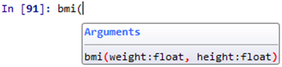
現在我們可以更清楚的看到需要輸入的內容型態。那如果我們還是胡亂輸入呢?比如不輸入數字反而輸入字串呢?這裡顯然會出現錯誤。不過其他函數也不一訂有錯,例如:
def greeting(name:str):
    print(f"Hello, {name}")
greeting([1,2,3])
這個函數要求輸入字串,但是我們輸入了list,不過程式還是執行了,當然或許你的名字就叫做[1,2,3],即使如此,正確的輸入方式還是greeting("[1,2,3]")。
當然我們可以在程式中再加入其他處理的手段,不過顯然這個anotation僅有提示的功能。Python的想法是大家都應該是成熟的人了,都已經跟你提示輸入型態了,還是硬要做錯誤輸入,不應該有這樣的幼稚行為。
-
Recap
- 如何給一個函數增加註解
- 如何查詢及使用函數的註解
第三十三話、Built-in Functions
之前提到好幾次Python的內建函數(Bifs),例如sum, min, max等,以下是所有bif的列表。| abs() | dict() | help() | min() | setattr() |
| all() | dir() | hex() | next() | slice() |
| any() | divmod() | id() | object() | sorted() |
| ascii() | enumerate() | input() | oct() | staticmethod() |
| bin() | eval() | int() | open() | str() |
| bool() | exec() | isinstance() | ord() | sum() |
| bytearray() | filter() | issubclass() | pow() | super() |
| bytes() | float() | iter() | print() | tuple() |
| callable() | format() | len() | property() | type() |
| chr() | frozenset() | list() | range() | vars() |
| classmethod() | getattr() | locals() | repr() | zip() |
| compile() | globals() | map() | reversed() | __import__() |
| complex() | hasattr() | max() | round() | |
| delattr() | hash() | memoryview() | set() |
help(abs)
print(abs(-10))
取得絕對值。就這樣。
-
Recap
- Built-in functions的列表
- 使用help查詢及使用built-in functions
第三十四話、Tuple
之前我們花了不少篇幅來介紹list,在此再介紹另一個資料結構(容器),tuple,這也是built-in functions中的一員。tuple的物件排列方式其實跟list一模一樣,也是一個串列,首先先來看一下tuple的help。help(tuple)根據這個介紹,我們可以使用以下幾個宣告tuple的方式。
tu1 = tuple()
tu2 = tuple([1,2,3])
tu3 = tuple((4,5,6))
print(tu1)
print(tu2)
print(tu3)
使用tuple()函數宣告的時候,無傳入參數表示宣告了一個空的tuple,若有參數則須是iterable,又因為tuple也是iterable,所以參數若為tuple則傳回該tuple。記得list還可以使用[]來表示,而tuple很顯然是使用()。所以也可以這樣宣告。
tu4 = ()
tu5 = (1,2,3)
tu6 = (1,)
print(tu4)
print(tu5)
print(tu6)
這裡特別舉了tu6這個例子,當tuple內僅有一個元素時,需要多加一個,號,來表示它是一個tuple,而不是一個數字,原因很簡單,如果沒有那個逗點,程式會認為小括號是用在運算而不是宣告tuple,所以型態會變成整數。
tuple跟list如此相像,許多的操作也類似。例如可以:
- 相加(+)
(1,2,3) + (4,5,6)
- 存取
tu2[1]
Note:注意要跟list一樣使用中括號來表示索引位置。 - 複製
tu2*3
- 切片
tu2[1:2]
- in跟not in
2 in tu2
1 not in tu2
- index & count
tu7 = tu3*3
print(tu7)
tu7.index(4)
tu7.count(5)
Note:index是傳回某個元素的索引值,而count則是計算在此資料結構的個數。這兩者在list並無介紹,不過list與tuple都能適用。 - 用for loop來traverse
for i in tu2:
    print(i)
看起來都一樣啊!到底差在哪裡?原來最大的差別便是tuple的內容是不可更動的(immutable),所以以下是不可操作的: - 改變元素內容
tu2[0] = 100
有一個情況似乎可以修改tuple內容,如下:tu8 = (1,2,[3,4]) tu8[2][1] = 100 print(tu8)
事實上並不算,它修改的是下下層內容。 - 刪除
del(tu2[:])
Note:不能刪除tuple內容,但是可以刪除掉整個變數,例如del(tu1)就可以。
這樣說起來,好像沒有tuple也無所謂,只要有list就可以了嘛!其實tuple在函數大概最好用的就是做為回傳值了。舉個簡單的例子。
def tupleTest(n:int)->tuple:
    return (n**2, n**0.5)
print(tupleTest(9))
這個函數傳回一個tuple,第一個元素是某數平方,第二個元素是某數的平方根。當函數要傳回不只一個資料時,便可以使用tuple。不過這樣的效果好像list也可以,倒也沒錯,不過tuple還有一個不同的功能,那就是可以直接分解為變數。使用剛剛的函數說明:
square, sroot = tupleTest(25)
print(square)
print(sroot)
本來函數傳回的是一個tuple,長這樣(平方,平方根)。兩個元素可以直接拆封成兩個變數(square, sroot)來取代。若是傳回是list,那就得說square =list[0],sroot=list[1],雖然效果可以相同,不過tuple比較容易使用。在一些語法中其實也用到這個概念,例如:
a,b = 1,2
print(a, b)
這可以快速宣告變數。之前提到的bifs中有一個函數名為divmod(),查一下它的介紹。
help(divmod)可以看到回傳值是一個tuple。所以可以這樣使用。
quotient, remainder = divmod(17,3)
print(quotient, " ", remainder)
原則上商就是17//3,而餘數就是17%3。應該不難吧。
-
Recap
- 如何宣告一個tuple
- tuple之相加、存取、複製、切片
- in & not in以及使用for loop進行traverse
- tuple內元素不能被更新以及刪除
- 使用tuple當作函數回傳值以及指派tuple元素給變數
第三十五話、Dict
dict是dictionary的簡寫,它跟list或tuple不同之處是不使用自動產生的索引值,而是須自己設計索引值。例如:dic1 = dict({1:"One", 5:"Five", 10:"Ten"}) print(dic1[1])使用dict()函數來建立dict,小括號內需為一個{},在:左方的是自訂索引值(key),右方的是對應的值(value),跟list類似的是在[]內給索引值即可。顯然dict在Python中的代表符號是{},所以也可以這樣宣告。
dic2 = {"one":1, "two":2, "three":3}
print(dic2["two"])
除此之外,還可以這樣宣告:
dic3 = dict([["j",11], ["q",12], ["k",13]])
print(dic3["q"])
小括號內是一個list,其中的元素只要是一對一對的list或是tuple都可以。Dict中的值是可以改變的,所以可以
dic3['k'] = 30
print(dic3)
我們可以觀察到dic3的內容順序是j,k,q,這是因為它會自動按照key來排序。那麼若是要新增資料進去一個dict怎麼辦?其實直接使用改變值的方法即可,只要給它新的key,例如:
dic3['a'] = 1
print(dic3)
因此,我們也可以這樣建立一個dict。
keys = list(range(1,10))
values = [x**2 for x in keys]
dic4 = {}
for i, k in enumerate(keys):
    dic4[k] = values[i]
print(dic4)
print(dic4[5])
所以如果我們可以有兩兩對應的值就可以直接建立dict了,因此只要能得到如下:
kv = [(k, values[i]) for i, k in enumerate(keys)]
print(kv)
那就可以產生dict了,
dic5 = dict(kv)
print(dic5)
或是這樣做
dic6 = {}
for k,v in kv:
    dic6[k] = v
print(dic6)
要取得兩兩對應的內容,也可以使用內建函數zip,例如:
for i in zip(keys, values):
    print(i)
因為zip()傳回的是一個zip物件,所以直接將其傳入dict()內可得:
dic7 = dict(zip(keys, values))
print(dic7)
順便多介紹一點zip的用法。
z1 = [1,2,3]
z2 = ('a','b','c')
z3 = (True, False, True)
zz = zip(z1,z2,z3)
for i in zz:
    print(i)
由上面例子可以看出來zip()函數可以接收多個輸入值(不定長度參數),並將這些輸入值(list or tuple)做另一方向的合併。請注意若是輸入的陣列長度不一樣,則zip的時候會取較短的長度做zip,其餘多的不做。
反過來說,如果有一個iterable物件,而其中的內容是類似zip後的內容,那麼我們可以進行unzip,例如:
kv = [(1, 1), (2, 4), (3, 9), (4, 16), (5, 25), (6, 36), (7, 49), (8, 64), (9, 81)]
d1, d2 = zip(*kv)
print(d1)
print(d2)
只要在iterable物件前面加上*號,表示要將其unzip。如果我們知道kv的元素之最短長度(使用len(kv[i])來檢測),那麼我們可以自己練習寫一個函數來進行upzip。
kv = [(1, 1), (2, 4), (3, 9), (4, 16), (5, 25), (6, 36), (7, 49), (8, 64), (9, 81)]
def unzip(zipped, sLen):
    uz = [[] for _ in range(sLen)]
    for v in kv:
        for i in range(len(uz)):
            uz[i].append(v[i])
    for j in range(len(uz)):
        uz[j] = tuple(uz[j])
    uz = tuple(uz)
    return uz
kv1, kv2 = unzip(k, 2)
print(kv1)
print(kv2)
-
Recap
- 如何宣告一個dict
- 如何新增資料到一個dict
- 如何使用函數zip()以及如何unzip
第三十六話、再話Dict
之前已經提到如何在dict內取得、修改或增加元素,那麼若是要刪除呢?我們可以使用del,例如:dict1 = dict([(1, 1), (2, 4), (3, 9), (4, 16), (5, 25), (6, 36), (7, 49), (8, 64), (9, 81)]) del(dict1[1]) print(dict1)若是要刪除的key並不包含在dict內,則傳回錯誤。
del(dict1[10])除了del之外,也可以使用popitem(),不過這個方法僅能刪除最後一個元素(最後一個表示最後一個加入dict的元素),若是要刪除某特定元素,則可使用pop(key),例如:
dict1.popitem()
print(dict1)
dict1.pop(4)
print(dict1)
與list類似,可以使用clear()來清除dict,使用del(dict)來刪除整個dict。
dict1.clear()
print(dict1)
del(dict1)
print(dict1)
在討論list的時候,我們示範了自己寫函數來清除list內容,那dict也能這樣做嗎?dict的索引值不像list有規律,那要怎麼辦?其實只要使用popitem()就可以了,如下:
dict1 = dict([(1, 1), (2, 4), (3, 9), (4, 16), (5, 25), (6, 36), (7, 49), (8, 64), (9, 81)])
for i in range(len(dict1)):
    dict1.popitem()
print(dict1)
那我們可以使用for loop來traverse一個dict嗎?首先我們要先了解dict的屬性,dict包含索引值(keys),對應數值(values),兩者合併的資料對(items),而這些屬性都有對應的方法可以得到。
dict1 = dict([(1, 1), (2, 4), (3, 9), (4, 16), (5, 25), (6, 36), (7, 49), (8, 64), (9, 81)])
print(dict1.keys())
print(dict1.values())
print(dict1.items())
keys(), values(), items()這三個方法可以分別傳回對應的iterable物件。所以我們可以根據他們來進行traverse,例如:
for k,v in dict1.items():
    print(f"{k}->{v}")
之前提到兩個list或是tuple可以使用+號合併,dict可以嗎?答案是不行的,我們可以寫個函數來相加兩個dict如下:
di_1 = {'a':1, 'b':2, 'c':3}
di_2 = {'one':1, 'two':2, 'three':3}
def addDict(dic1, dic2):
    for k in dic2.keys():
        dic1[k] = dic2[k]
    return dic1
di_3 = addDict(di_1, di_2)
print(di_3)
一樣的效果可以使用dict的方法update()來完成。
di_1 = {'a':1, 'b':2, 'c':3}
di_2 = {'one':1, 'two':2, 'three':3}
di_1.update(di_2)
print(di_1)
沒甚麼困難的。不過我們感興趣的是,如果兩個dict中有重複的key,那會怎樣?
di_1 = {'a':1, 'b':2, 'c':3}
di_2 = {'one':1, 'two':2, 'c':100}
di_1.update(di_2)
print(di_1)
好吧!看起來是以dic2為主,也就是說要解釋為用dic2來更新dic1。
說到這裡,再回鍋說一下函數的annotations,當我們建立了一個有annotations的函數,我們可以得到annotations的資料嗎?答案是肯定的,資料儲存在__annotations__這個變數內,所以我們可以這樣做(使用之前的bmi()函數):
bmi.__annotations__
咦,原來是個dict。所以我們顯然可以如此得到相關資訊。
bmi.__annotations__['return']
-
Recap
- 刪除dict內元素,可以使用del、popitem、pop,使用clear()刪除所有資料
- 使用dict之keys()、values()、items()來取得對應的資料
- 相加兩個dict,使用update()函數
- 函數的annotations由__annotations__參數取得,是為一dict
第三十七話、未定關鍵字參數函數
再次回頭討論一下函數。之前提到未定長度參數函數,可以傳入函數不定個數的參數,這裡要談的未定關鍵字參數(Arbitrary keyword arguments)也是類似,可以傳入函數隨意個數keyword arguments。在表示的時候,使用雙星號(**),先看一下以下的例子:def arbitrary(**kwargs): print(kwargs) arbitrary(one = 1, two = 2, three = 3)這個函數甚麼都沒有,就只是把參數印出來,顯示出來kargs是一個dict。原來所謂的Arbitrary keyword arguments就是把傳入的參數放進一個dict內,再看一個例子。
def aveScore(**scores): for k, v in scores.items(): ave = sum(v)/len(v) print(f"class {k}'s average score is {ave}") aveScore(class101=[78, 88, 98], class102=[88, 79, 85], class103=[81, 98, 78])也可以直接傳入一個dict:
classes = {"class101":[78, 88, 98], "class102":[88, 79, 85], "class103":[81, 98, 78]} aveScore(**classes)要記得在傳入的dict前面加上**才行。看起來蠻方便的,那若是與其他類型的參數合用怎麼辦?估計未定關鍵字參數應該要放在最後面。我們可以大致上遵循這樣的順序:
- positional arguments
- variable number of arguments (*args)
- keyword arguments
- Arbitrary keyword arguments (**kwargs)
def healthExam(name, age, *dates, bloodType=None, **others): print(f"{name}, {age}, Exam Dates:{dates}, Blood Type:{bloodType}", end="") for k, v in others.items(): print(f", {k}:{v}",end="") print("\n") healthExam("Tom", 18, "10/1", "7/19", bloodType="A") healthExam("Mary", 20, "1/16", "12/9", bloodType="B", �'張�"=88, �"�縮�"=123)顯示結果如下:
Tom, 18, Exam Dates:('10/1', '7/19'), Blood Type:A
Mary, 20, Exam Dates:('1/16', '12/9'), Blood Type:B, 舒張壓:88, 收縮壓:123
A piece of cake☻。
除了上述的幾種輸入參數用法之外,再介紹一種用法,叫做keyword-only arguments。意思是這種參數僅能使用關鍵字,而不能使用positional arguments來代替。先舉一個我們已經會的例子:
def arcLength(arcid = 0, x1 = 0, y1 = 0, x2 = 0, y2 = 0): length = ((x1-x2)**2 + (y1-y2)**2)**0.5 return f"arc id = {arcid} length = {length}" a = arcLength("AB", 1, 3, 10, 20) print(a)我想這個求線段長度的函數對你來說應該是桌上拿柑一般的容易。我們確實可以用positional arguments的傳入方式來使用裡面的所有參數。不過如果我們希望在呼叫函數時,部分參數強制使用keyword(稱為keyword-only arguments),那怎麼辦?強制使用的好處是清楚明瞭,比較不會搞混。而做法就是在這些參數的前面加上一個獨立的*號,如下例。
def arcLength(arcid = 0, *, x1 = 0, y1 = 0, x2 = 0, y2 = 0): length = ((x1-x2)**2 + (y1-y2)**2)**0.5 return f"arc id = {arcid} length = {length}" a = arcLength("AB", x1 = 1, y1 = 3, x2 = 10, y2 = 20) print(a)可以看到在arcid之後加了一個獨立的*號,表示在*號之後的所有參數都得使用keyword傳入數值,如果在呼叫函數時有一個沒有使用keyword,就會產生錯誤。例如這樣呼叫:
a = arcLength("AB", 1, y1 = 3, x2 = 10, y2 = 20)特別提醒一下,keyword-only arguments不依定需要有預設值,例如:
def koTest(a, b, *, c, d): print(f"{a},{b},{c}, {d}") koTest(1,2,c=3,d=4)這樣是可以的。我們可以把*視作將參數分為兩區的符號,兩區各自獨立運作,所以這樣設計也可以。
def koTest(a, b = 0, *, c = 0, d): print(f"{a},{b},{c},{d}") koTest(1,2,c=3,d=4)本來沒有初始值的參數d是不能排在有初始值的參數之後的,但是因為*號之後的參數強制使用keyword來傳入,所以就沒差了。
-
Recap
- 使用**kwargs來定義未定關鍵字參數,參數儲存在一個dict內
- 依照特定順序來設計不同種類參數可使用所有四種參數
- 使用,*,來定義keyword-only參數,此參數僅能使用keyword傳入
第三十八話、函數夢話
之前提到函數也可以當作函數的傳回值,那麼函數可否是函數的傳入參數呢?來試試看。def funArg(fun, arr): arr = [fun(x) for x in arr] return arr newArr1 = funArg(lambda x:x**2, [1,2,3,4,5]) print(f"newArr1 = {newArr1}") newArr2 = funArg(lambda x:x**0.5, [1,2,3,4,5]) print(f"newArr2 = {newArr2}")嘿,是可以的,只要給一個函數再給一個list,funArg()就會把這個函數應用在list的每一個元素上。這是一個強力好用的功能,不過各位大概也猜到Python是否也已經有這樣的函數,你猜對了,那就是內建函數map(),其用法如下:
alist = [x for x in range(1,6)] list(map(lambda x: x**2, alist))一樣給函數跟list,不過因為傳回的是map物件,所以將它cast成為list再來觀察。我們來把事情搞複雜一點,如果map裡面的函數它的輸入值也是函數,這樣行嗎?
s = lambda x: x**2 r = lambda x: x**0.5 aList = [s, r] for i in range(1,6): output = list(map(lambda f: f(i), aList)) print(f"i = {i} -> {output}")這個例子中,alist包含兩個函數,所以在使用map()時,每次都將這兩個函數分別傳入要用來map的函數,也就是上例的f得到的是一個函數,輸出的解如下:
i = 1 -> [1, 1.0]
i = 2 -> [4, 1.4142135623730951]
i = 3 -> [9, 1.7320508075688772]
i = 4 -> [16, 2.0]
i = 5 -> [25, 2.23606797749979]
另一個類似的內建函數為filter(),這個函數的目的是讓我們過濾list內的部分元素,用法如下:
blist = [3, -5, -7, 12, 8, -10, 9, -1] list(filter(lambda x: x<0, blist))很明顯可以看出來只有x<0才是要保留的,而x>0的就被過濾了。依照慣例,我們自己設計個函數來試試看。
def filter2(func, arr): newList = [] for i in arr: if func(i): newList.append(i) return newList testList = [3, -5, -7, 12, 8, -10, 9, -1] print(filter2(lambda x: x < 0, testList))EZ!最後再介紹一個函數,它的功用是將陣列內的元素逐一往下計算,比方說有一個list是[1,2,3,4,5],我們想要給一個包含兩個參數的函數來表示list中前後元素需做的計算,一路到底,最後傳回一個值(不是list),例如是兩數相加的函數,則算法是先1+2,然後計算(1+2)+3,然後計算(1+2+3)+4,最後計算(1+2+3+4)+5可以得到所有元素的總和。函數的寫法如下:
def reduce2(func, arr): temp = arr[0] for i in range(1, len(arr)): temp = func(temp, arr[i]) return temp rList = [1,2,3,4,5] result = reduce2(lambda x,y: x+y, rList) print(f"result = {result}")執行程式後可以看到答案是15。不過說起來好像這個函數很廢,我們隨意地用個sum(rList)就可以得到答案了不是?不過如果改一下輸入的函數參數就比較不同了,例如:
reduce2(lambda x,y:x*y, rList)這可以得到相乘的結果。又或者
reduce2(lambda x,y:x/y, rList)相除的結果(等同於1/2/3/4/5)。當然各位又會猜測是不是又有一個內建函數可以做相同的事?答案不是,有這樣一個函數名為reduce,但它不是built-in function,它被收納在functools這個模組內,所以要使用時須先將其納入,語法如下:
from functools import reduce reduce(lambda x,y:x+y, rList)只要記得先加上from functools import reduce這一行,其用法跟我們自己設計的函數一模一樣。至於import的相關用法後面再介紹。
-
Recap
- 了解map()、filter()、reduce()的用法
- 練習自己定義與上述函數相同內涵的函數
第三十九話、函數之老生常談
到這裡大致上學會了設計函數的所有基本概念及方式,想要熟悉程式設計,沒有甚麼新鮮的好方法,多做練習來增加熟練度總是需要的。所以這裡來做個練習並總結一下。首先假設有兩個list(xs, ys),各自包含9個數字(int),甚麼數字其實不重要,假設xs包含1-9,ys包含與xs對應數字的平方。要做的事情是:- 將xs與ys的對應數字做成數字對(也對應x,y座標),儲存於一個list內
- 設計一個函數計算兩點間距離
- 將前一個數字對與後一個數字對代入現段距離的函數
- 儲存前後兩點距離並將其儲存在一個list。
- 計算所有線段總距離並將其印出
def dis(*, x1:float, y1:float, x2:float, y2:float)->float: """ 計算兩點間距離 """ return ((x1-x2)**2+(y1-y2)**2)**0.5 xs = [x for x in range(1,10)] ys = list(map(lambda y: y**2, xs)) print(f"所有x座標\n{xs}\n對應y座標\n{ys}") xy = list(zip(xs, ys)) print(f"每一個點的座標\n{xy}") arcLength = [] for e in range(len(xy)-1): arcLength.append(dis(x1=xy[e][0], y1=xy[e][1], x2=xy[e+1][0], y2=xy[e+1][1])) print(f"前後點形成的線之長度\n{arcLength}") from functools import reduce totalLength = reduce(lambda a,b: a+b, arcLength) print(f"線段總長度={totalLength}")
第四十話、set
我們已經學過了list、tuple、以及dict三種基本的容器,這裡再介紹另一種,set。Set其實跟list或是tuple類似,也是串接的資料,最大的不同處是如果資料有重複的物件,set內僅會保留一個,也就是說set內不會有重複的物件。而其宣告的函數則為set(),快速使用符號為大括號{}。不過大括號不就已經是dict的專利了嗎?因為dict需要成對資訊,但是set的內容比較像list或tuple,所以可以得出分別。但是要注意如果要宣告一個空白的set,就不能僅使用大括號{},那是因為程式會誤認為我們要宣告的是一個dict。例如:dict1 = {} type(dict1) set1 = set({}) type(set1)不是空白的set宣告就可以直接使用大括號了,如下:
set2 = {'a','b','c'} type(set2)其他的資料結構可以使用set()函數來cast。
list1 = [1,3,5,2,4,5,6,3] set(list1)很明顯可以看出list1轉換成為一個set,而其中的元素僅留下不相同的內容。比較有趣的是這個例子:
set("one little two little three little Idians")當放入的是字串時,會取得組成的字母集合(因為字串算是一種的list)。所以set可以理解成組合成某集合所需要之最基本元素之組合。
若是要在一個set內新增資料,可以使用add()函數。
set1 = {1,2,3} set1.add(4) print(set1) set1.add(2) print(set1)add()一個新元素沒有問題,之前做過許多類似的了,只是在set內add一個本來就存在的元素時的反應才是我們感興趣的,不過在意料之內,結果是沒反應,因為反正加進去也會被整理成只剩一個。
那若是要刪除呢?若是要刪除的是元素,使用remove(x)或是discard(x),兩者的差別是若是x不包含於set內,remove(x)會傳回錯誤。例如:
set1 = {1,2,3} set1.remove(1) set1.discard(2) set1.discard(5) set1.remove(5)若是不想要看到錯誤,顯然得使用discard()或是使用remove()但是先檢查該元素是否存在,例如:
if 5 in set1: set1.remove(5) else: print("Does not contain 5")還可以使用pop()來刪除元素,不過set不像list或是tuple可以使用[index]來取得元素,所以pop()這個函數只好隨機刪除某一元素,例如:
set3 = set("Python is not difficult.") print(set3) set3.pop() set3.pop()我們可以觀察到上面的set其實是根據大小順序排序的,但是pop時確實是隨機的。不過在測試數字時,卻又根據排序順序刪除,看這個例子:
set10 = {5,3,9,1,8,2,0} print(set10) set10.pop() set10.pop() set10.pop() set10.pop()蠻怪的,還是就當它是隨機刪除的好了。此外,若是要刪除所有元素,一樣,使用clear()。
set10.clear() print(set10) del(set10) print(set10)這都跟其他的容器一樣,使用clear()清空,使用del(set)刪除整個set。
-
Recap
- 了解set的宣告方式及基本內涵(其內元素無法更改及刪除)
- 使用add()函數新增元素
- 使用discard()、remove()、pop()、及clear()來移除元素
- 使用del()來刪除set
第四十一話、set的運算
set除了保留基本元素之外,主要的重點就是集合的運算。跟數學的集合一樣,我們可以求得交集聯集等新集合。首先來看交集。set1 = {1,2,3,4,5} set2 = {1,3,5,7,9} set1 & set2 set1.intersection(set2)交集就是在A且在B,所以使用&,也可以使用intersection()這個方法。而聯集就是在A或在B,可以使用|或是union(),如下:
set1 | set2 set1.union(set2)特別提醒在使用intersection()或是union()時,傳入參數可以不一定是set,也可以是list或是tuple,例如:
set1.union([2,4,6,8])聯集不是使用+號,不過差集卻是使用-號(或是使用difference()方法),所謂差集就是在A但不在B,例如:
set3 = {1,2,3,4,5} set4 = {4,5,6,7,8} set3 - set4 set3.difference(set4)差集可以使用A-(A&B)來驗算,如下:
set3 - (set3 & set4)最後一個,XOR就是在A或在B但不在A&B,運算符號為^(或使用symmetric_difference()方法),驗算方式就是(A|B)-(A&B),如下例。
set3 ^ set4 set3.symmetric_difference(set4) (set3|set4)-(set3&set4)再次提醒,difference()與symmetric_difference()都可以使用其他容器例如list或tuple等做為輸入參數。
除了這幾個基本的集合運算,set還包含數個方法,我們可以使用help(set)來查詢,這裡再介紹幾個方法或操作,其餘各位可自行練習。
- 判斷交集是否為空集合,使用isdisjoint()
set1.isdisjoint(set2)
- 判斷集合是否為某集合的子集合,使用<或<=或issubset()
{1,2} < {1,2,3,4,5}
- 判斷集合是否為某集合的母集合,使用>或>=或issuperset()
{1,3,5,7,9}.issuperset({3,5,7})
- 雖說不能使用A+B來將兩個集合合併,不過可以使用update()方法
set1 = {1,2,3,4,5} set2 = {1,3,5,7,9} set1.update(set2) print(set1)
雖然好像出現跟set1|set2一樣結果的集合,不過聯集是產生新的集合,而update是使用另一個集合更新原集合(本來集合變成聯集內容,也就是原集合被更新),效果並不完全相同。 - 指派運算子(|=、&=、-=與^=)
這應該不用多說了,例如A&=B就是A=A&B的意思。
set5 = {1,2,3} set6 = {2,4,6,8} set5 &= set6 print(set5)
print([x for x in range(2,20) for y in range(2,x) if (x%y==0)])這個寫法可以得到2到20間不是質數的數,當然有重複的內容,不過不怕,因為我們有set。
print(set([x for x in range(2,20) for y in range(2,x) if (x%y==0)]))再來就容易了,我們只要算出包含2-20元素集合與此集合的差集即可。
set(range(2,20))-(set([x for x in range(2,20) for y in range(2,x) if (x%y==0)]))雖然囉嗦了一點,不過還是可以利用集合的運算來得到質數。此外,之前提的list comprehensive也可以用在set內,所以上式可以再簡短一些。
set(range(2,20))-{x for x in range(2,20) for y in range(2,x) if (x%y==0)}
-
Recap
- 了解set的運算:交集(A&B)、聯集(A|B)、差集(A-B)、以及XOR(A^B)
- 了解isdisjoint()、issubset()、issuperset()、update()等方法之用法
第四十二話、Frozenset
基本的內建容器架構大多介紹了,再說一個Frozenset,顧名思義,這就是一個set,最大的不同處是frozenset是不可變動的,例如:fset = frozenset({1,2,3,4,5,5,4,3,2,1}) print(fset) fset.add(6)Oops!不能新增。原則上|=, &=, -=, ^=, add(x), remove(x), discard(x), pop(), 以及clear()都不能用在frozenset。那這個frozenset到底有甚麼用?先看一下這個例子:
set1 = {1,2,3,4,5} set2 = {6} set1.add(set2)之前倒沒試過這個,看來set內是不能包含另一個set。此時frozenset上場了,再看看這個例子:
fset1 = frozenset({6}) set1.add(fset1) print(set1)一個set可以包含frozenset。好像就沒甚麼好說的了,frozenset還是可以做交集聯集等集合運算,只是傳回變成frozenset,例如:
fset = {1,2,3,4,5} anotherset = {4,5,6,7} sets = {fset|anotherset, fset&anotherset, fset-anotherset, fset^anotherset} print(sets)如上所述,set可以包含fronzenset,而frozenset就是一個不可變動(immutable)的set,就好像tuple就是一個不可變動的list一般。
-
Recap
- 了解frozenset的宣告方式
- Frozenset是immutable
- Frozenset可以為set之元素,但set不可為set之元素
第四十三話、再說字串
又回頭來談談字串。字串就是一串的字元,因為常是資料內容或運算結果,常會遇到需要操作或運算它的場合,所以在此特別介紹。字串由字元組成,原則上它就是一個list,不過跟list的操作有一點點小小的不同,我們先看這個例子:s = "Time is money." print(s[1]) s[1] = 'o'當我們使用list的方式取得其中元素時,是可以的,但是當我們要指派值的時候,是不行的,也就是說字串也是immutable。不過其他許多list的操作倒是都可以,例如:
for i in s: print(f"{i}", end=" ")雖說字串是一種list,卻又有點不一樣,我們用這個方式來將字串真的變成一個list。
ss = [] for i in s: ss.append(i) print(ss)這個部分顯然對各位是沒問題的,有趣的是我們能夠把字串list轉化為我們想要的字串嗎?當然可以,此時需要的是join()這個函數。這個函數的輸入參數是連結的字串,看了例子便明白。
print(",".join(ss)) print("".join(ss)) print("|".join(ss))使用一個字串把list中的每個元素連起來,變成另一個字串。接下來介紹一些字串的操作:
- 切片(slicing)
這原則上就是list的功能了,做個練習。
s[8:-1]
好吧,不需要滿腦子都是money。 - 裁剪(strip, lstrip, rstrip)
裁剪的意思是將字串兩端(注意是兩端,跟中間部分無關)的空白去掉,例如:
s = ' This is a str. ' len(s) s = s.strip() print(s) len(s)
若是僅想去掉左邊或右邊的空白,則使用lstrip或rstrip,這部分請自行練習。函數strip在接受使用者輸入指令或資料時很有用,有些使用者會不小心在兩端多輸入了空白,這個時候我們就可以將其裁剪來避免錯誤。除了去除空白之外,strip還可以去除字串,例如:s = 'This is a str' s.strip('str')
事實上只要字串前後有與strip()內的參數相同的字串,都會被清除,例如:s.strip('aTbctderf')
上例中因為Ttr三個字與s的前後相符,因此前後的字母被裁剪了。 - 分割(split, rsplit, partition, rpartition)
當我們有一個字串,有一些場合會需要將其分割來萃取其中的部份資訊,此時可使用split。例如:
record = "001, KaoHsiung, New York, papers, 2018/12/31" record.split()
假設我們有一筆資料如上(事實上我們常會有一大堆類似格式的資料),此時我們可以將其中每個部分的內容分割開來形成一個list,接下來我們想要使用哪一部分的資料就隨心所欲了。如果我們使用help查詢split這個方法,可以得到如下資訊:help(str.split)
其實我們可以輸入兩個參數進入split這個方法,第一個sep就是要用來分割的字串(預設值是空白),第二個maxsplit就是要拆解的次數。所以再看這個例子:s = "Time is money." s.split(maxsplit=1)
因為沒給sep,所以使用預設值也就是空白,而maxsplit=1的意思就是只拆一次(形成兩個元素),所以is money就沒有被分割。應該很清楚了,rsplit就沒甚麼好說的了,它只是從右邊往左邊分割罷了。Split的sep並不會被保留,例如:s.split("i", maxsplit=1)
若是我們想要保留set使其成為list中的一員,則可以使用partition,如下:s.partition("i") s.partition("is") s.partition("m")
不過要注意的是partition僅能分割一次,也就是說在字串中找到第一個(自左往右)符合sep的字串,然後將字串分為三部分,也就是sep的左邊,sep本身,以及sep的右邊(好像把木頭切成兩半,切了後剩三部分,左邊的木頭,右邊的木頭,以及中間的木屑)。要注意的是partition()傳回的是tuple而不是list。至於rpartition就是由右邊開始,沒甚麼好著墨的。如果字串並不包含sep,那使用split()或partition()會怎麼反應? ☻s.partition("was") s.split("was")
- 計數(count)
可計算某子字串(substring)出現的次數。例如:
s = "Time is money." s.count("is") s.count("i")
- 首尾字串(startswith, endswith)
判斷字串是否以某字串開頭或結尾,例如:
s.startswith("Ti") s.endswith("ney.")
也可以用來判斷子字串,只要註明子字串的位置,例如:s.startswith("mo", 8, -1) s.endswith("ney", 8, -1) s[8:-1]
不知不覺中又只關注在money。
-
Recap
- 字串是list,也是immutable
- 使用for loop將字串傳換成list,使用join()將字串list轉換成字串
- 字串可以切片(slicing)
- 使用strip()去除字串兩端空白,使用split()與partition()分割字串
- 使用count()計算子字串的出現次數,使用startswith, endswith來判斷是否以某特定字串作為開頭或結尾
第四十四話、字串接著說
因為不想讓一話的篇幅太長,所以拆成兩話,這算是split嗎?- 尋找(find, rfind, index, rindex)
Find是自左往右找到第一個符合的子字串位置(傳回index),rfind自然是由右往左。
s = "Time is money." s.find("money")
尋找位置(index)也是自左往右在字串內找到參數字串位置(還記得這個方法在list跟tuple都有嗎?),但與find不同之處為若字串並不包含該子字串,則傳回錯誤(ValueError)。例如:s.index("money") s.index("cash")
rindex不用再說了吧。 - 大小寫轉換(upper, lower, capitalize, swapcase, isupper, islower, casefold)
小寫變大寫(upper)、大寫變小寫(lower)、首字母大寫(capitalize)、大小寫互換(swapcase)、判斷是否大寫或小寫(isupper、islower),不囉嗦,直接使用。
s.upper() s.lower() s.capitalize() s.swapcase() s.isupper() s.islower()
至於casefold(),測試了一下就是變成小寫,如下:s.casefold().isupper() s.casefold().islower
不過不管它,如果兩個字串都是casefold(),比較時便可以不計大小寫。似乎都使用lower()也是一樣,不過casefold()是比較強的版本,因為也可用於其他語言。 - 判斷內容(isalpha, isdecimal, isdigit, isnumeric,isalnum, isspace)
- 判斷是否為字母(isalpha) – 若包含space傳回False
s1 = "abc" s1.isalpha() s2 = "123" s2.isalpha()
- 判斷是否為整數(isdecimal),是否為整數數字與上下標數字的unicode(isdigit),是否為整數數字、上下標數字與分數的unicode(isnumeric)
s2.isdecimal() s3 = "12.3" s3.isdecimal() s4 = "2\u00b2" print(s4) s4.isdigit() s5 = '2\u2082' print(s5) s6 = "\u00bd" print(s6) s6.isnumeric()
- 判斷是否包含字串及數字(isalnum)
s7 = "a1" s7.isalnum()
- 判斷是否是空白字串(isspace) – space、tab(\t)、return(\n)都算
s8 = " \t" s8.isspace()
- 判斷是否為字母(isalpha) – 若包含space傳回False
- 置中(center)
Center的輸入參數是總長度,也就是字串會放在這個長度範圍的中間。
s9 = "center" s9.center(20)
重寫我們在loop時學的三角星陣。for i in range(1,10): print(('* '*(10-i)).center(20))
- 填滿(zfill, ljust, rjust)
zfill()表示將多出來的空白用0填滿。
s.zfill(30)
ljust表示原字串靠左,填滿右邊;rjust表示原字串靠右,填滿左邊。例如:s = "This is a str." s.ljust(30, '#') s.rjust(30, '#')
- 轉換(maketrans,translate)與代換(replace)
轉換有兩個函數Maketrans與translate,兩者通常是合併使用,先使用maketrans定義一個轉換表,再將轉換表當作translate的參數來進行轉換。在使用maketrans函數時,如果只輸入一個參數,必須是一個dict包含著unicode或字元對應unicode或字串。若是輸入兩個參數,必須是相等長度的字串,才能對應。例如:
x = 'aeiou' y = '12345' table = str.maketrans(x,y) s = 'This is a str.' s.translate(table)
或是例如:dic = {'2':'\u2082', '3':'\u2083'} table = str.maketrans(dic) "H2O2 + CaCO3".translate(table)
代換(replace)是將字串中的某一子字串用另一個新的字串取代。例如:s = 'This is a str.' s.replace('is', 'xy')
Replace如果輸入第三個參數(整數)是代表自左到右的代換次數,例如:s = 'This is a str.' s.replace('is', 'at', 1)
-
Recap
- 使用find, rfind, index, rindex來搜尋字串
- 使用upper, lower, capitalize, swapcase, isupper, islower, casefold來轉換或判斷大小寫
- 使用isalpha, isdecimal, isdigit, isnumeric,isalnum, isspace來判斷字串內容
- 使用center來將字串置中
- 使用maketrans,translate來轉換、使用replace來代換
Python亂談
物件
第四十五話、import
之前我們學過了使用Built-in function,也學會了自己設計函數,接下來我們想要使用別人寫好的函數。為了方便工作,程式設計師會把許多有關的函數放在一起,稱為模組(module),當需要使用的時候把這個模組導入,就可以使用了。不需要重新設計又可以重複使用(當然可以給其他人使用,例如我們)。有些模組需要額外安裝,當然有許多在我們安裝IDE的時候就同時安裝了,我們只需要使用import這個關鍵字就可以將其導入然後開始使用了。千言萬語不如舉個例子,我們先舉math這個例子說明。Math這個模組顧名思義就是數學相關的函數,當我們要使用時這樣做。import math help(math)當使用help()後,會出現一大串函數,此時我們已經可以使用了。選其中一個函數試試看,例如pow(x,y),傳回x的y次方,等同於x**y。
math.pow(2,5)在我們欲使用這個模組中的函數時,語法是模組名.函數名(),這樣程式就了解我們要呼叫某模組內的某函數了。
接下來我們打開另一個console,
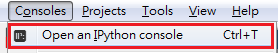
點下去後會出現Console 2/A,先在此console內打help(math),將會發現出現錯誤,那是因為我們還沒有將此模組導入。好吧,到底現在要說甚麼呢?假設我們想要有一個函數可以開根號,我們也知道在math這個模組內有一個函數sqrt()可以用來開根號,我們只想要導入sqrt()這個函數,其他的函數並不需要,那我們可以這麼做。
from math import sqrt sqrt(9)這個意思就是從(from)math這個模組導入(import)sqrt這個函數。接下來我們可以直接使用sqrt()這個函數了。請注意此時不是使用math.sqrt()。
當我們使用import math的時候,math稱為namespace,在使用pow()這個函數時,我們需要先註明這是來自math這個模組的函數,如果你還有印象,其實built-in function內也有一個pow()函數,所以其實我們可以看到這樣的結果(回到Console 1/A)。
math.pow(2,5) pow(2,5)這表示這是兩個不同的函數。所以儘管我們可以這麼做(回到Console 2/A),
from math import * pow(2,5) sin(1)*號是wild card(跟撲克牌的鬼牌類似),代表全部。當這樣導入時,我們不需要強調math這個模組的名稱便可直接使用其內的函數,但是在使用pow()這個函數時卻無法分別到底是在使用哪一個函數。若是發生同名但是不同內容的情況就不是我們樂見的。所以,我們應該避免使用from 模組 import *這樣的導入方式,因為有namespace可以讓我們更清楚的分別我們在呼叫哪一個函數(好比有兩個人都叫做阿花,我們要強調是張家的阿花還是李家的阿花才知道是哪一個人)。
接下來再看一個例子,假設我們要導入另一個模組random,顯然這是跟隨機數有關的模組,如果我們使用import random,這當然可以,之後就使用random.函數名()這樣的語法來使用其內的函數。不過random這個名字有點長,每次輸入有點累,可否讓它縮短一些?可以,語法如下:
import random as rd help(rd)此時random的namespace名稱為rd,所以要使用help()查詢時,要給的名稱是rd,若是使用random則出現錯誤,因為這麼名稱電腦不認得(已經改名為rd了),因為random這個模組的內容太長,所以按下去後找不到上面的輸入了,你可以自己試試看。As這個關鍵字英文解釋是作為,以……的身分;當作,應該不難理解。我個人覺得或許也可以解釋為alias這個字的縮寫,也就是使用後面的名稱來當作模組的別名,不過不重要,記得用as改名比較重要。
現在我們了解如何導入模組了,即使是常用的模組(每個人的常用定義不同),也有一大堆的函數,所以我們不再像介紹字串一般大肆介紹,親愛的你要自己花時間去了解怎麼使用,在你需要使用的時候便可以使用,老話一句,要花時間練習。不過既然導入了random,我們來寫個小程式練習回顧一下。random適合用在許多研究或是設計遊戲,現在我們來練習個猜拳遊戲,寫在Talk45_1.py這個檔案內。
import random as rd yourGuess = input("請出拳(scissor, paper, stone)") if rd.random() <1/3: computer = "scissor" elif 1/3 <= rd.random() <2/3: computer = "paper" else: computer = "stone" yourGuess = yourGuess.strip().casefold() if computer.casefold() == "scissor".casefold(): if yourGuess == "scissor".casefold(): print(f"It's a Tie(you:{yourGuess} com:{computer})") elif yourGuess == "paper".casefold(): print(f"You Lose(you:{yourGuess} com:{computer})") else: print(f"You Win(you:{yourGuess} com:{computer})") elif computer.casefold() == "paper".casefold(): if yourGuess == "scissor".casefold(): print(f"You Win(you:{yourGuess} com:{computer})") elif yourGuess == "paper".casefold(): print(f"It's a Tie(you:{yourGuess} com:{computer})") else: print(f"You Lose(you:{yourGuess} com:{computer})") else: # computer==stone if yourGuess == "scissor".casefold(): print(f"You Lose(you:{yourGuess} com:{computer})") elif yourGuess == "paper".casefold(): print(f"You Win(you:{yourGuess} com:{computer})") else: print(f"It's a Tie(you:{yourGuess} com:{computer})")順便回顧一下字串的用法,現在你輸入隨意大小寫的剪刀石頭布,都可以正常地玩了。不過這個程式猜一次就會停止,如果你想要猜三次或是猜到想停為止,你知道怎麼做的。 提到import,順道提一下這個指令:
import this
The Zen of Python, by Tim PetersBeautiful is better than ugly.
Explicit is better than implicit.
Simple is better than complex.
Complex is better than complicated.
Flat is better than nested.
Sparse is better than dense.
Readability counts.
Special cases aren't special enough to break the rules.
Although practicality beats purity.
Errors should never pass silently.
Unless explicitly silenced.
In the face of ambiguity, refuse the temptation to guess.
There should be one-- and preferably only one --obvious way to do it.
Although that way may not be obvious at first unless you're Dutch.
Now is better than never.
Although never is often better than *right* now.
If the implementation is hard to explain, it's a bad idea.
If the implementation is easy to explain, it may be a good idea.
Namespaces are one honking great idea -- let's do more of those!
這稱為Python之禪,是提供在撰寫程式時的一些想法準則跟意境,你可以自己感受一下。
-
Talk45_1.py
- 使用import或是from module import function來導入
- 使用import module as md來導入並改名
- 勿使用from module import *來導入
Recap
第四十六話、物件
Python算是一個物件導向的程式語言(Object-Oriented Programming, OOP),其內的物品都是物件。到底甚麼是物件,就是一種東西的類型,可以包含變數與方法。好像有聽懂了,又好像有點模糊,依照慣例來舉例說明(Talk46_1.py)。假設我們有以下資料:math = [89,68,98,73,71] eng = [77,91,83,75,66] python = [78,80,83,92,69]這是某班級同學的數學英文與程式的成績。如果我們想知道某位同學平均成績,可以使用例如math[2]+eng[2]+python[2]/3來求得,這沒有問題。不過這位同學叫甚麼名字?我們需要另一個儲存名字的list,例如:
name = ["大雄","胖虎","小夫","靜香","小杉"]如此這般,name[2]就是我們要的答案。不過我們若是先問班上同學數學自高到低的排列是為何?那就是要排序,我們可以選擇list的方法sort()或是使用built-in function中的sorted()皆可。sort()之前用過了,這裡用sorted()試試看。
math = sorted(math, reverse=True) print(math)如果這個步驟先做了,現在要問靜香的平均分數就麻煩了,次序全亂了。若是每一人的資料綁在一起就好了,像這樣:
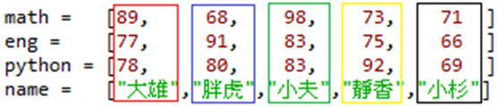
在這其中,即使內容不同,每一個人都有一個名字三個分數,只要我們設計一個模式,裡面是包含這幾個屬性就可以了,此時我們可以使用關鍵字class,如下:
class One(): math = None eng = None python = None name = None這表示有一類型(class)的物品稱之為One,將來每一個One都包含著四個屬性。我們可以根據這個class來產生一個物件,並且可以指派每一個屬性的值,例如:
one_0 = One() one_0.math = math[0] one_0.eng = eng[0] one_0.python = python[0] one_0.name = name[0]接下來我們可以將內容印出來看看。
print(f"Name:{one_0.name},Math:{one_0.math},Eng:{one_0.eng},Python:{one_0.python}")看得出來可以使用one_0屬性這樣的語法來取得屬性值。這個one_0就稱為物件(instance),而class One就是這類型物件的設計圖。有了這個設計圖,我們可以有任意數量的物件,例如:
one_3 = One() one_3.math = math[3] one_3.eng = eng[3] one_3.python = python[3] one_3.name = name[3] print(f"Name:{one_3.name},Math:{one_3.math},Eng:{one_3.eng},Python:{one_3.python}")每次建立一個新的物件,在記憶體中就會配置一塊空間,給這個物件使用,就好像之前我們宣告變數一樣,只是物件需要的空間可能大許多罷了,當我們使用物件名.變數名這樣的語法,便可以分別要取得的變數是在哪一個物件內的變數,他們指稱的是不同塊的記憶體。有了物件後,現在要得到任一人的平均都不會麻煩了,因為只要知道物件名,就不會搞錯了。不過每一個人(物件)都要算一次類似
ave3 = (one_3.math + one_3.eng + one_3.python)/3 print(ave3)這樣的步驟,又有點麻煩,若是有一個函數來幫忙就好了。確實可以在class內設計函數,稱之為方法,只要能夠取得class內的變數的值就好了。這話是甚麼意思?變數不就是在class內嗎?以上例來說,如果在class內說math,拿到的是變數math還是外面的list math?因應這樣的情況,即使我們改變變數的名稱,也不能直接取得,Python使用關鍵字self稱呼每個物件自己,所以self.math才是指的class內的變數math,因此我們可以設計方法如下:
math = [89, 68, 98, 73, 71 ] eng = [77, 91, 83, 75, 66 ] python = [78, 80, 83, 92, 69 ] name = ["大雄","胖虎","小夫","靜香","小杉"] class One(): math = None eng = None python = None name = None def ave(self): """ 計算平均分數 """ return (self.math+self.eng+self.python)/3 one_3 = One() one_3.math = math[3] one_3.eng = eng[3] one_3.python = python[3] one_3.name = name[3] print(f"{one_3.name}的平均分數為{one_3.ave()}")執行後可以得到平均分數。而且也可以使用help(One.ave)或help(one_3.ave)來查詢ave這個方法。
help(one_3.ave)此時class的雛型已經成形了,One()就像int()、list()等,每宣告一次,便傳回給你一個物件。
接下來我們又覺得每次都要一一指派值給每一個變數太麻煩,可不可以使用輕便一點的方法,反正每次一開始就要給值不是嗎?沒值寸步難行啊。所以,我們設計一個方法,在我們宣告時,直接給值,這一個方法稱為初始化,而且它有固定的名稱,叫做__init__()。
class One(object): def __init__(self, math, eng, python, name, theClass = "101"): self.math = math self.eng = eng self.python = python self.name = name self.theClass = theClass def ave(self): """ 計算平均分數 """ return (self.math+self.eng+self.python)/3 one_4 = One(math[4], eng[4], python[4], name[4]) print(f"{one_4.name}的平均分數為{one_4.ave()}")注意,總結一下,class內的方法第一個參數都要是self,表示是自己,物件自己的變數,也都要用self來指代,表示是自己的變數,__init__後小括號內的是傳入參數,也就是傳入這些值,並將他們指派給class內變數。順帶一提,在One()之後的小括號內有一個object,這是表示class One是繼承自object,,也就是說這個物件是繼承自object,因為object就是所有物件的共同祖先。__init__主要用於建構,但也是一個方法,所以跟一般函數一樣可以有預設值參數,例如如果我們在__init__()輸入參數內加上theClass="101"來表示班級,那在宣告時班級的預設值當然是101。
再稍微提一下self,self指的是物件本身,如果我們建立一個class如下:
class Whatever: def what(): print(f"What?")其實我們可以直接使用其中的方法:
Whatever.what()這樣的方法又稱為static method,也就是可以直接使用class名來呼叫方法。可是當我們建立物件如下:
w = Whatever() w.what()因為當我們使用w.what()時,內定我們必須將自己當作第一個傳入變數,所以在設計的時候,方法的第一個變數須為self。而且有了self,就可以使用class內的變數,因為self指的就是這個class,例如:
class Whatever: name = "Tom" def what(self): print(f"What? {self.name}")此時用這兩個形式都可以呼叫what(),
Whatever.what(Whatever)或
w = Whatever() w.what()可見使用instance呼叫class內方法,傳入自己是預設值,而且方法若沒有傳入self,就無法取得class內的name參數,所以變成慣例,內建self當作第一個傳入參數。
-
Talk46_1.py
- Class為物件的設計圖,instance為根據設計圖所產生之物件
- 使用關鍵字self來指稱物件自己
- Class內可以包含__init__()方法來做為初始化的根據
Recap
第四十七話、物件之屬性
再繼續前面的例子,class內有個方法,我們可以使用help(One)來查詢物件資訊或使用help(One.ave)來查詢方法資訊。如果查詢help(__init__)也可以得到建構子的資料。事實上class的屬性也可以後來再加上,例如:cedar = One(math[4], eng[4], python[4], name[4]) cedar.physics = 72此時cedar擁有physics這個變數屬性,可以存取資料,但是class架構沒有,其他的物件也沒有。
help(cedar.__init__)如果我們在console打上以下指令:
print(cedar)沒甚麼資訊,只跟我們說cedar是個物件,那要怎麼顯示物件內容?要顯示的內容當然我們自己訂,只要增加一個方法__str__()即可。
def __str__(self): return (f'{self.name}的math={self.math}, eng = {self.eng}, python={self.python}')重新執行後在console輸入:
print(cedar)有了,跟平常使用的變數字串一樣。不過通常我們不用print()也有資訊,這是怎麼來的?若要這個效果,需要在class再加上另一個方法:
def __repr__(self): return (f'{self.name}的math={self.math}, eng = {self.eng}, python={self.python}')顯然這個方法的內容與__str__內容相同,不過其使用時機不同,為直接在console輸入cedar所顯示的內容。
原來在Python中有一些定義好的方法名稱,是對應console內的指令用途的。如上例__str__就是給print()顯示用的資料,__repr__就是給直接顯示變數內容使用的。只要使用help(tom)就可以檢查有哪些內容,之前我們在談幫變數命名時提到,有這些內定的名稱前後有兩底線的,是應該在命名時避免的。那除了__init__及這兩個還有那些其他常用的內建方法呢?
- __getattr__()
當我們要查詢class內的屬性(變數或方法)時,通常使用cedar.math這樣的語法,不過如果我們查詢了一個不存在的屬性呢?例如cedar.music,會出現甚麼?
cedar.music此時若是不想要這個錯誤,那可建立這個方法__getattr__()。def __getattr__(self, name): print(f"Looking for {name}?") return None
有沒有return None倒是不重要。之前提到我們可以自己外加參數屬性,所以如果偵測到沒有屬性,那倒是可以做點事。if cedar.music is None: cedar.music = 60 print(cedar.music)
在外加參數屬性時,可以先行判斷是否已存在。 - __getattribute__()
首先先介紹一個參數,__dict__。
print(cedar.__dict__)
__dict__是一個dict,其內儲存了class所有的變數及其值。當我們要得到屬性值時,使用cedar.math,便是呼叫__getattribute__(),然後查詢cedar.__dict__["math"]的值,因此我們不需要建立這個方法。原則上它的內容如下:def __getattribute__(self, name): return object.__getattribute__(self, name)
因為__getattribute__()就是查詢__dict__[],所以不能傳回self.__dict__[name],這樣會造成無窮迴圈。 - __setattr__()
很顯然這是要設定屬性值的,只要把值給__dict__s內的對應item即可,也是不需要自行建立。其內容如下:
def __setattr__(self, name, value): print(f"改變{name}的值為{value}") self.__dict__[name] = value
不需要印出這行字,這裡只是測試,你會看到每次改變都有提示。 - __setitem__() & __getitem__()
假設我們的屬性中有一個dict(或是list亦可),在此例中包含一些學科分數,我們可以使用cedar['music']這樣的方式來存取資料。作法就是加上這兩個方法:
def __setitem__(self, key, value): self.grade[key] = value def __getitem__(self, key): return self.grade[key]
記得要加上self.grade = {}這個屬性。cedar['music'] = 99 print(cedar['music'])
其實等同於print(cedar.grade['music'])
我們可以使用cedar.__dict__來查看內容。 - __call__()
這個方法可以讓我們使用instance直接呼叫。例如:
def __call__(self, math, eng, python, name, theClass = "101"): self.math = math self.eng = eng self.python = python self.name = name self.theClass = theClass self.ave()
現在可以使用物件直接呼叫方法,也就是呼叫__call__()方法。cedar(89,91,75,"Dora") print(cedar)
我把__getattr__, __setattr__, __getattribute__三個方法comment掉,免得出現太多訊息。 - __name__ 這個參數其實若只是單獨寫一個程式是用不到的,不過若是要導入其它模組就可能需要了,因為導入時就開始執行。所以被導入時,__name__是模組名稱,若是直接執行,則它的值等於'__main__',所以通常使用__name__=="__main__"來判斷是否直接執行。
-
Talk47_1.py
- Class的屬性可以在建立後再加入
- __str__跟__repr__讓我們顯示class訊息
- __getattr__, __setattr__, __getattribute__可以讀取屬性
- __setitem__與__getitem__可直接操作class的dict參數
- __call__可使用instance直接呼叫
Recap
第四十八話、getters & setters
本來想繼續用前一話的例子,不過好像越來越長了,還是再寫一個新的。這次的物件使用蜘蛛人。class SpiderMan(object): ''' class of spider man ''' def __init__(self, age): self.age = age def __str__(self): return f"Age = {self.age}" def __repr__(self): return f"Age = {self.age}"這沒有甚麼問題,只要輸入一個變數即可初始化。
peter = SpiderMan(22) print(peter)我們已知可以直接使用peter.age = 23來賦值,不過有個問題,如果我們給的是以下的值呢?
peter.age = -10 print(peter) peter.age = "隨便啦" print(peter)這並不是我們樂見的。因此,通常我們希望避免出現這樣的問題,賦值與取值都使用方法來代替,在方法中我們便可以做些限制或修正,一般來說賦值的方法前面都會加個set,取值的方法都會加個get,所以這些方法統稱為getters and setters。現在把剛剛的class修改一下:
def __init__(self, age): self.age = None def setAge(self, a): if type(a) != int: print("Error: age has to be an integer.") elif a < 0: print("Error: age has to be positive.") else: self.age = a def getAge(self): return self.age然後執行:
peter = SpiderMan() peter.setAge(-22) peter.setAge("22")現在若是輸入非正整數的值,都會出現錯誤訊息。也可以使用Python的關鍵字assert(聲稱、斷言、堅持)來控制輸入值,將方法改為如下:
def setAge(self, a): assert type(a)==int and a > 0, "age has to be an integer and > 0" self.age = a很明顯assert之後的是聲稱堅持的條件,逗點之後的是錯誤訊息,此時輸入不合理的值會出現如下錯誤訊息。
peter = SpiderMan() peter.setAge("20")這方式會迫使程式中斷,直到輸入正確為止。
當我們使用getter&setter來存取設定變數時,如果不想要變數被直接使用,那可以在變數之前加上一個底線,例如我們在class內加上一個新的變數_weight,然後加上以下兩個方法:
def setWeight(self, w): assert type(w)==float and w > 0, "weight has to be a positive float." self._weight = w def getWeight(self): return self._weight weight = property(getWeight, setWeight, doc = "spiderman's weight')執行後再使用會出現怎樣的情況?
peter.weight = 70.1 peter.weight peter._weight = 71.1 peter._weight這樣是看不出來甚麼,因為在class內的變數是_weight,但是我們又知道可以在事後定義class的變數,所以看起來我們應該現在有兩個變數,weight與_weight。但是因為加上了property()這個物件來定義weight,使得當我們使用peter.weight時,實際上是在呼叫setWeight()或getWeight()方法。所以接著看以下操作:
peter.__dict__ peter.weight is peter._weight事實上class內僅有一個變數。如果本來我們設計了一個class變數但是沒有getters&setters,但是後來又改變主意,加上了getters&setters,此時所有存取變數的instance可能都要修改(e.g. 將peter.weight改為peter.getWeight()),但是如果我們這樣做的話,就不需要改變了,可以繼續使用peter.weight。
在上例中,即使使用了getters&setters,我們還是可以直接使用peter.age來改變其值,這樣設計getters&setters好像沒有甚麼用。例如:
peter.age = -8 peter.__dict__如果要強調不能直接使用變數(也就是須經過getters&setters才能調用),我們可以在變數前面加上兩條底線,例如再加上一個變數稱為__salary,然後加上以下方法:
def setSalary(self, s): assert type(s)==float and s > 0, "salary has to be a positive float." self.__salary = s def getSalary(self): return self.__salary執行程式後,輸入以下指令:
peter = SpiderMan() peter.setSalary(50000.0) peter.getSalary() peter.__salary這樣的做法可以將參數封裝,但是Python內號稱是沒有private變數的,看一下內容:
peter.__dict__
其實__salary用_SpiderMan__salary這樣的方式儲存了,所以其實還是能夠直接改變它。
peter._SpiderMan__salary = 80000.0 peter.getSalary()雖然無法完全避免自外直接修改它,至少讓我們知道他是很重要的變數,我們不希望它被修改。
-
Talk48_1.py
- 使用getters&setters來控制變數值的輸入
- 使用底線+變數及property()來設計變數使得變數可直接取得getters&setters方法
- 使用雙底線+變數來封裝變數,避免直接改變變數
Recap
第四十九話、物件的比較
我們已知在Python內的東西都是物件,而當我們輸入1<2,會傳回True。這表示兩個物件可以比較大小,當然兩個值都是數字來比大小對我們來說確實沒有問題。若是"A"<"B"呢?還是可以的,傳回一個True。不過如果我們自訂一個class,建立兩個物件(instance),這樣還是可以比較大小嗎?兩台電腦誰大誰小?兩輛車怎麼樣算大或小?原則上我們學過可以比大小的是有自然排列順序的東西,例如數字、字母。其他東西的比較,就等我們自己定義。套用上一話的SpiderMan來做例子,為了方便測試,把__init__修改一下並另存為Talk49_1.py。兩個spider man比大小,如果說我們是要根據其體重好了,那我們可以這樣做。
peter = SpiderMan() peter.weight = 70.1 mary = SpiderMan() mary.weight = 50.2 peter.weight > mary.weight好像有比較大小了,不過跟我們想像中的不大一樣,可否使用peter > mary或是peter==mary呢?此時我們需要設計相關的方法如下:
- __gt__(>)、__lt__(<)、__ge__(>=)、__le__(<=)
def __gt__(self, other): if self._weight > other._weight: return True else: return False
當設計了__gt__(>)之後,(<)就自動可以使用了。不過在檔案中還是都寫了相關方法,__ge__與__le__跟(>)(<)類似,只是多了等號,設計這個你絕對沒有問題的。 - __eq__(==)
在我們設計是否相等之前,先看一下以下指令。
peter = SpiderMan(_weight = 70.0) mary = SpiderMan(_weight = 50.0) peter == mary mary.weight = 70.0 peter == mary
即使沒有設計__eq__方法,本來我們就可以使用==(!=)來判斷是否相等(或不等)了,此時跟使用is判斷是等同的。所以如果要依我們自己的標準來判斷是否相同,需要重寫__eq__方法。根據之前的邏輯,判斷是否相等(或不等),好像直接照著改就行了。def __eq__(self, other): if self._weight == other._weight: return True else: return False
使用起來也沒問題。peter = SpiderMan(_weight = 70.0) mary = SpiderMan(_weight = 50.0) peter == mary peter != mary
不過我們怎麼知道mary是不是spider man,如果她是Wonder woman可以嗎?先設計一個簡單的class WonderWoman。class WonderWoman(object): def __init__(self, _weight = None): self._weight = _weight def setWeight(self, w): assert type(w)==float and w > 0, "weight has to be a positive float." self._weight = w def getWeight(self): return self._weight weight = property(getWeight, setWeight, doc = "WonderWoman's weight")
接下來再比較:peter = SpiderMan(_weight = 70.0) mary = WonderWoman(_weight = 70.0) peter == mary
這就變得有點怪了,依照這個邏輯,若是有一個物件是腳踏車,只要重量相同,相比之後也會相等。若是我們的標準,要相同的物件才能比較,那就得先判斷兩物件是否屬於同一類,做法如下:def __eq__(self, other): #if isinstance(other, type(self)): if isinstance(other, self.__class__): return self._weight == other._weight else: return False
-
Talk49_1.py
- 設計__gt__(>)、__lt__(<)、__ge__(>=)、__le__(<=)、__eq__(==)等方法來判斷兩物件之關係
- 使用isinstance(obj, class)來判斷某物件是否為某class之instance
Recap
第五十話、例外處理
雖然我們小心翼翼,苦心孤詣的設計程式讓它沒有錯誤,但是在某些情況下還是會產生我們意料之內的錯誤,我們知道這個錯誤在某些情況下可能會發生,所以我們必須先行處理它。為什麼我們不能直接讓它不發生呢?請看以下例子:while True: age = int(input("你今年幾歲?")) if age < 0: break else: print(f"你今年是{age}歲了。")執行後輸入abc,會出現錯誤。其實如果使用者都乖乖地輸入數字,是不會有錯誤的,但是意料之內,總是會有人輸入非數字來讓它出現錯誤(+.+),此時我們可以做點甚麼嗎?根據上面的錯誤內容,可以看出來是出現了ValueError,所以我們可以使用關鍵字try...except…..來處理它,如下:
while True: try: age = int(input("你今年幾歲?")) if age < 0: break else: print(f"你今年是{age}歲了。") except ValueError: print("正確的輸入須為整數")白話文翻譯,我們試著(try)做這些指令,當出現了某一種錯誤(ValueError),則執行except ValueError之下的指令。那麼如果可能發生超過一個的錯誤呢?例如:
def reciprocal(): x = float(input("請輸入一個數字:")) return f"{x}的倒數為{1/x}" r = reciprocal() print(r)很顯然跟之前一樣我們也不應該輸入文字,但是即使是輸入數字0,還是錯的。嗯,表示我們預見可能會有兩種錯誤發生,此時try...except...的寫法如下:
def reciprocal(): try: x = float(input("請輸入一個數字:")) return f"{x}的倒數為{1/x}" except (ValueError, ZeroDivisionError): print("輸入值須為數字不為0") r = reciprocal() print(r)這樣可以了,兩種例外都偵測得到,可見excep後面可以使用tuple,然後將可能的錯誤列上去。不過這樣可能就不知道是發生哪一個錯誤了,所以也可以分開寫,如下:
def reciprocal(): try: x = float(input("請輸入一個數字:")) return f"{x}的倒數為{1/x}" except ValueError: print("輸入值須為數字") except ZeroDivisionError: print("輸入值不可為0") r = reciprocal() print(r)這樣就可以偵測不同的錯誤了。Python顯然內建了許多例外型態,那我們怎麼記得了那麼多?第一個方法就是多看多用就會多記得了,到這個網頁可以看到相關列表https://docs.python.org/3/library/exceptions.html。此外,真的不知道也懶得查,也就是只想要混過去的話,可以使用wild card(鬼牌),不過這是不好的,應盡量避免。如下:
def reciprocal(): try: x = float(input("請輸入一個數字:")) return f"{x}的倒數為{1/x}" except: print("有錯誤發生") r = reciprocal() print(r)雖然這樣可以抓到例外,但是卻不知道是甚麼例外,對於使用者幫助不大,所以最好把知道的錯誤都寫上去,最後才再加上except,這樣會比較好一些。
Try…except…還可以跟else及finally兩個關鍵字連用,else內的指令是在沒有發生例外時執行,而finally內的指令則是最後一定會執行。將上例修改如下:
def reciprocal(): try: x = float(input("請輸入一個數字:")) except ValueError: print("輸入值須為數字") except ZeroDivisionError: print("輸入值不可為0") except: print("發生未知錯誤") else: return f"{x}的倒數為{1/x}" finally: print("執行完畢") r = reciprocal() print(r)在設計方法時,若預見會出現錯誤,也可以使用raise來提出。例如:
class SuperMan(object): def __init__(self, _age = None, name = None): self._age = _age self.name = name def setAge(self, a): if not isinstance(a, int): raise ValueError(a) else: self._age = a def getAge(self): return self._age age = property(getAge, setAge, doc = "superman's age")當出現錯誤情形時,將強制提出錯誤。執行以下指令。
clark = SuperMan(name = "Clark Kent") clark.age = "18"因為輸入不正確的值,所以直接出現錯誤。因為在設計方法時就預見會出現這個錯誤,所以在之後使用時,便知道要處理它,因此若是欲使用這個class內的方法,可以寫像如下的方式:
if __name__ == '__main__': clark = SuperMan(name = "Clark Kent") try: clark.age = "18" except ValueError: print("年齡須為整數") else: print(f"{clark.name} is {clark.age} years old.") finally: print("Super!")因為我們已經知道要使用clark.age = '18'可能出現ValueError,所以放進try內,並且隨時偵測是否出現錯誤。
-
Talk50_1.py
- 使用try…except…來處理發生的錯誤,可以處理超過一個錯誤
- 可以與else及finally連用(optional)
- 可以使用raise在可能發生錯誤之處提出
Recap
第五十一話、繼承
之前我們提過在設計class時,class名後面的小括號是要繼承的物件(之前都是object)。當一個class(稱為subclass或child class)繼承另一個class(稱為superclass或parent class),subclass會獲得superclass的全部屬性,好比父母遺傳給兒女。所以如果我們想要設計一個class,又發現這個class可以是另一個class的翻版再加上一些變化,那麼便可以使用繼承(inherit)了。舉個例子來說明:class Vehicle(object): def __init__(self, maxSpeed): self.maxSpeed = maxSpeed def setSpeed(self, s): self.maxSpeed = s def getSpeed(self): return self.maxSpeed def __repr__(self): return f"車輛最大速度為{self.maxSpeed}" __str__ = __repr__這是車輛的雛型,只有一個最大速度的變數。若是接著我們想要設計一個腳踏車的class,顯然腳踏車也是一種車,所以可以繼承自vehicle,如下:
class Bicycle(Vehicle): def __init__(self, maxSpeed, power): Vehicle.__init__(self, maxSpeed) ### <<< self.power = power self.type = "腳踏車" def setPower(self, p): self.power = p def getPower(self): return self.power def __repr__(self): return f"{self.type}的最大速度為{self.maxSpeed},動力為{self.power}" __str__=__repr__註解標示處表示在初始這個class時,也呼叫初始Vehicle這個class的方法,這樣我們就可以將其納入。若是我們試著建立此class的instance,則跟之前的class沒有差別。
b1 = Bicycle(40, "人力") print(b1)要注意的是Vehicle與Bicycle都包含__repr__這個方法,在使用時,subclass會覆寫superclass的同名方法,稱為overriding。現在若是還想要建立一個單輪車的class,那顯然可以繼承腳踏車,如下:
class UniCycle(Bicycle): def __init__(self, maxSpeed, power, capacity): Bicycle.__init__(self, maxSpeed, power) self.capacity = capacity self.type = "獨輪車" def setCapacity(self, c): self.capacity = c def getCapacity(self): return self.capacity def __repr__(self): return f"{super().__repr__()},可載{self.capacity}人" __str__ = __repr__執行後可見:
u1 = UniCycle(10, "人力", 1) print(u1)類似的道理也可以用於Vehicle->Car->Truck等,新的class原則上我們會新增函數或方法,因為畢竟是新的物品,應該有新的屬性。在__repr__()內,使用了super()這個函數,這個函數的意義就是superclass,所以super().__repr__()就是呼叫父類別的__repr__()方法。類似的內容我們就不需要多做一次。接著我們來看以下兩個class:
class ArmoredCar(Vehicle): def __init__(self, maxSpeed, armor): Vehicle.__init__(self, maxSpeed) self.armor = armor self.type = "裝甲車" def setArmor(self, a): self.armor = a def getArmor(self): return self.armor def __repr__(self): return f"{self.type}最大速度為{self.maxSpeed},{self.armor}" __str__=__repr__和
class Artillery(object): def __init__(self, caliber): self.caliber = caliber def setCaliber(self, c): self.caliber = c def getCaliber(self): return self.caliber def fire(self): print("Fire!!") def __repr__(self): return f"火炮的口徑為{self.caliber}mm" __str__=__repr____ArmoredCar是有裝甲的車輛,繼承自Vehicle,Artillery是火炮,有一個屬性是口徑,這兩個的組合是甚麼?答案是蝙蝠車(Batmobile)。問題是要怎麼產生一個新的class是來自兩個class的組合,這樣的形式稱為多重繼承(multiple inheritance)。做法如下:
class Batmobile(ArmoredCar, Artillery): def __init__(self, maxSpeed, armor, caliber): super().__init__(maxSpeed, armor) #self.caliber = caliber >> 此行與下行擇一皆可 Artillery.setCaliber(self, caliber) self.type="蝙蝠車" super().fire() def __repr__(self): return f"{super().__repr__()},{Artillery.__repr__(self)}" __str__=__repr__首先可以看到Batmobile繼承自兩個class,所以兩個都寫上去,用逗號分開。接著看到在__init__內使用super(),有兩個要super哪一個?總有個是主要的,答案是第一個(如果super()要呼叫的方法在第一個superclass內並沒有,則在第二個superclass內找,例如fire()這個方法)。而第二個可以使用上述的兩種方式,任選一個。在__repr__內也是一樣,super()指第一個,另一個則使用class名稱來取得。如果要繼承三個class也是一樣,主要的super()是指第一個。執行的結果如下:
bm = Batmobile(80, "防彈裝甲", 50) print(bm)上一話我們提到例外的處理,如果我們想要自己定義自己的例外,可以繼承自Exception這個class,例如:
class AgeLessThanZeroError(Exception): def __init__(self, age): self.age = age def __repr__(self): return f"Error:年齡小於0: {self.age}" __str__=__repr__將這個class應用到之前的SuperMan這個class,如下:
class SuperMan(object): def __init__(self, _age = None, name = None): self._age = _age self.name = name def setAge(self, a): if not isinstance(a, int): raise ValueError(a) else: if a < 0: raise AgeLessThanZeroError(a) else: self._age = a def getAge(self): return self._age age = property(getAge, setAge, doc = "superman's age")執行後如下:
sm = SuperMan(name = "Clark Kent") sm.age = -18
-
Talk51_1.py
- 將superclass之名寫在subclass的名稱後小括號內
- 使用super()取得superclass
- 多重繼承將superclasses都寫入小括號內,以逗點隔開,此時super()將自第一個superclass開始尋找使用
Recap
第五十二話、繼承的限制與Overriding
之前我們提過在變數前面加一底線與加二底線會有甚麼不同,含糊一點的說,沒有底線的可稱為public,加一底線稱為protected,加二底線則稱為private,那在繼承時會有差別嗎?做個例子試試看。class Car(object): color = "Black" _year = 2019 __price = 1000000 def __repr__(self): return f"Color: {self.color}, Year:{self._year}, price: {self.__price}"再設計一個:
class Benz(Car): moonWindow = True def __repr__(self): return f"{super().__repr__()}, Moon Window:{self.moonWindow}"在console建立物件如下:
benz = Benz() benz.color benz._year benz.__price加上兩底線的變數無法被繼承,當然我們之前就知道如果硬是要得到內容還是有辦法的:
benz._Car__price
不過這件事不應該常做,算是特殊手段。現在再把class Benz修改如下:
class Benz(Car): moonWindow = True color = "Silver" _year = 2018 __price = 3000000 def __repr__(self): return f"{super().__repr__()}, Moon Window:{self.moonWindow}"接著執行:
benz = Benz() benz因為__repr__內的金額是由super()得來的,所以沒有被改變,因為無法繼承private,現在把__repr__修改如下:
def __repr__(self): return f"{super().__repr__()}, Moon Window:{self.moonWindow}, New Price:{self.__price}"再執行一次:
benz = Benz() benz現在變成兩塊記憶體分別記載著不同的價錢,如下:
benz._Benz__price benz._Car__price至於何謂Overriding?其實很容易,上例中的__repr__就是overriding,當在subclass定義一個與superclass同名不同內容的方法,之後subclass的instance呼叫方法時,使用的是現在subclass內的方法,而不是繼承得來的方法,因為該方法已經被覆蓋。好像這樣就說完了,還是弄個例子好了,分別在上述兩個class內各建立一個同名的方法,例如:
def deprecation(self, year): return self.__price*0.1*year這是一般汽車的折舊率。
def deprecation(self, year): return self.__price*0.05*year這是Benz的折舊率。數字是我瞎掰的,真實的折舊率請自行研究查詢。那麼當Benz的instance呼叫deprecation(),是使用繼承而來的還是現有的,答案很明顯了。
benz = Benz() benz.deprecation(1)如果想使用superclass的方法,只要使用super()即可,例如再加上這個方法到class Benz:
def compareDeprecation(self): print(super().deprecation(1), " ", self.deprecation(1))現在測試看看:
benz = Benz() benz.compareDeprecation()之前提到的都是變數,好像沒有說到如果是方法的話是不是一樣。原則上是相同的,在方法名前面加上雙底線,也會讓它變成private,進而無法繼承,例如:
class superc(object): def __pri(self): print("This is a private method") class subc(superc): pass若是建立一個subc來使用__pri(),結果如下:
c = subc() print(c.__pri())加兩底線的private方法無法繼承使用,那有沒有其他用處?看一下以下例子:
class superc(object): def __init__(self, listb): self.lista = [] self.__update(listb) def update(self, listb): for i in listb: self.lista.append(i) class subc(superc): def update(self, courses, scores): for i in zip(courses, scores): self.lista.append(i) info = ["Tom", 18] s = subc(info) course = ["Python","Java"] score = [99, 95] s.update(course, score) print(s.lista)這個例子中,superc內有一個lista,這是存放學生資料的list,在初始的時候會呼叫update這個方法,將傳入資訊寫入lista。不過在繼承自superc的subc內,也有一個update方法來override前一個class內的方法,此時的update()內的傳入參數與superc內的不同,因此,若是執行此程式會出現錯誤。這怎麼辦?其實可以將subc內的方法改名就好了(例如改為update_)。不過這樣要更新資料(update)就會出現多個名字,容易搞混,那另一個方法就是讓superc裡面的操作是private,這樣不會繼承下來,就不會互相干擾了。做法如下:
class superc(object): def __init__(self, listb): self.lista = [] self.__update(listb) def update(self, listb): for i in listb: self.lista.append(i) __update = update只要改superc就可以了。也就是說在superc內建立兩個一模一樣內容的方法,一個private自己用,一個不是private給繼承的class隨意override。執行結果會如下:
['Tom', 18, ('Python', 99), ('Java', 95)]
-
Talk52_1.py
- __變數名這樣命名的變數在繼承時無法被繼承
- 可以使用_className__變數名來取得private變數
- Overriding是使用目前的方法覆蓋superclass內的同名方法
- __方法名也是private,一樣無法被繼承
Recap
第五十三話、物件的老生常談
再來練習一下。題目如下: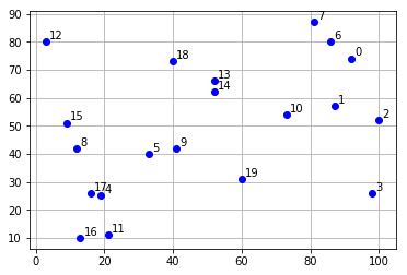
假設在100*100的平面上有20個點(編號0-19),座標使用random模組產生,如下:
import random as rd rd.seed(20) x = [rd.randint(0, 100) for _ in range(20)] y = [rd.randint(0, 100) for _ in range(20)]其中的seed()意思是在產生隨機變數時,給一個種子,根據這個種子,每一此產生的系列隨機數都會相同。也就是不管執行這個程式幾次,每次產生出來的x,y內容都相同。如果我們改變種子,例如將20改為10,那就會產生另一序列的隨機數,但是只要不改變種子,就會重複產生相同的序列。這個用意是固定題目,如果沒有seed,那麼每次產生的題目就都會不一樣,這樣就無從比較起。而第0點的座標就是(x[0], y[0])了,依此類推。
我們要求的是如果有一個路徑從某一點出發,經過其他所有點一次且僅有一次,最後又回到出發點,那總距離是多長呢?想像每一個點是一個商店,出發點是倉庫,車子從倉庫出發到每一點去送貨,最後又回到倉庫,這樣的路線有多長?當然這裡我們並不介紹怎麼找到很好的路徑,我們僅專注在怎麼求得路線長度,所以路徑就隨機產生。因為有很多點,所以首先來建立點的class:
class Node(object): def __init__(self, nodeid, x, y): self.nodeid = nodeid self.x = x self.y = y def __repr__(self): return f"id = {self.nodeid}, x = {self.x}, y = {self.y}" __str__ = __repr__接下來可以根據這個class產生instance,剛好有20個,我們將其儲存在一個list內。
nodes = [] for i in range(len(x)): nodes.append(Node(i, x[i], y[i]))可以先執行一下看看nodes裡面的內容:
print(nodes)跟我們想像的一樣。接下來可以先計算如果路線就是list內的物件順序的話路線長度是多少?意思就是從第0點到第1點到第2點…要記得最後要回到第0點。根據這樣的需求,我們設計以下兩個函數,第一個是兩點間距離的函數,這應該沒問題,之前寫過類似的,只是這次的輸入參數是兩個點,如下:
def distance(a:Node, b:Node)->float: """ 計算兩點a,b之間的直線距離 """ return ((a.x-b.x)**2+(a.y-b.y)**2)**0.5接下來設計另一個函數,輸入一個list,list內的點的排列順序就是路徑的順序,如下:
def totalLength(route:list)->float: """ 計算儲存在route内的路徑總距離 """ tLen = 0 for i in range(len(route)-1): tLen = tLen + distance(route[i], route[i+1]) # 再加上回程的長度 tLen = tLen + distance(route[-1], route[0]) return tLen因為每一次要抓到兩個點來計算,所以n個點只能算n-1次,因此要讓次數等於len(route)-1,以免超過list長度。最後再加上回程的距離,這樣就可以算出總長度。再測試一下:
totalLength(nodes)接下來我們要將nodes這個list裡面的物件排列順序打亂,使用的是shuffle這個方法,它可以將list內的順序打亂重排。看一下help:
help(rd.shuffle)測試一下這個方法:
rd.shuffle(nodes) nodes確實可以打亂,現在我們讓這個list打亂然後求得總距離20次好了,但是我們要記錄下來總距離最短的那次。做法如下:
rd.seed() # rd.seed(None) for i in range(20): if i==0: rd.shuffle(nodes) minLength = totalLength(nodes) minList = deepcopy(nodes) else: rd.shuffle(nodes) newLength = totalLength(nodes) if newLength < minLength: minLength = newLength minList = deepcopy(nodes)首先使用rd.seed()來將種子設定為空,若是還有seed,那麼之後的shuffle又會遵循一樣的序列,我們希望的是之後的shuffle每一輪都會不同。將最佳路徑及路徑長度分別儲存在minList及minLength兩個變數中,只要找到更好的解,就更新。記得要使用deepcopy必須要加上from copy import deepcopy才能使用。
這樣雖然完成了整個作業,不過整個程式看起來其實有點亂,所以我將其重新整理成Talk53_2.py的模樣。這裡將整個城市分為兩個class,第一個還是Node,第二個class為Route,初始的時候定義nodes、minLength、minList,
def __init__(self, nNodes = 20): self.nNodes = nNodes self.nodes = [] self.minLength = None self.minList = None self.initializeNodes()而distance()與totalLength()都定義為class內的方法,因為在class內,記得其第一個傳入參數要為self,且在其中呼叫其他class內方法也都要改為self.方法名。
此外再定義一個方法稱為newRoute(),在這裡接收傳入參數times做為執行次數,
def newRoute(self, times): rd.seed() # rd.seed(None) for i in range(times): if i==0: rd.shuffle(self.nodes) self.minLength = self.totalLength(self.nodes) self.minList = deepcopy(self.nodes) else: rd.shuffle(self.nodes) newLength = self.totalLength(self.nodes) if newLength < self.minLength: self.minLength = newLength self.minList = deepcopy(self.nodes)找到的最佳解直接儲存在minLength、minList兩個class變數內。
最後在主程式的部分(if __name__=="__main__":)建構一個Route物件然後呼叫newRoute()即可得到答案。
if __name__=="__main__": nnodes = 20 # number of nodes in the problem iteration = 20 # number of iteration route = Route(nnodes) route.newRoute(iteration) print(f"minList = {route.minList} \nminLength = {route.minLength}") route.plotFigure()在class Route內另外定義了一個plotFigure()方法,這是用來繪製最佳解的圖的方法,看不懂請勿擔心,之後會提到。
-
Talk53_1.py
Talk53_2.py
- 將程式內容分割整理為不同class與method,可以讓架構比較清楚,容易理解與維護
Recap
第五十四話、自訂import
我們可以在指令列(console)輸入指令,但當關機後便找不到你之前定義變數、函數或物件了。所以我們學會將指令寫在檔案(稱為script)內。如果是需要重複使用的一段內容,我們可以將其寫成函數(function)或是建立物件,如果是常用的函數或物件呢?那我們將其寫成另一個檔案,稱為module,若要使用時,直接將其import來使用。一個module原則上就是一個python(.py)的檔案。舉個例子說明。首先在一個檔案內(module1.py)加上以下內容:
pi = 3.14159 def CircleArea(radius): return pi*radius*radius def TriangleArea(bottom, height): return bottom*height/2接著再開啟主要要工作的檔案(Talk54_1.py),因為要import所以要將這兩個檔案放在同一個資料夾才行。內容如下:
import module1 as m1 radius = 10 print(f"Radius = {radius} >> Area is {m1.CircleArea(radius)}")跟之前import其他模組的用法相同,讚。( ͡° ͜ʖ ͡°)
討論一下,在module1中,有一個變數是pi,不過其實我們可以在其中import math,然後得到math.pi來代替pi。意思就是在module中,我們還是可以再import其他的module,module拉module,環環相扣。
接著我們再建立另一個module,稱為module2.py,都放在同一個資料夾內。裡面就簡單放個class如下:
class polygon(object): def __init__(self, sides): self.sides = sides def __repr__(self): return f"A polygon with {self.sides} sides"這時在主檔案內加入如下指令:
import module2 as m2 p3 = m2.polygon(3) print(p3)嗯哼,果然得到我們預期的效果☜(⌒▽⌒)☞。如果也想知道這個三角形的面積,當然我們知道怎麼加上一個方法來計算。不過我們在module1的時候不是定義過面積的方法了嗎?拿來用?那就把module2修改如下:
import module1 as m1 class polygon(object): def __init__(self, sides, a = None, b = None): self.sides = sides self.a = a self.b = b def area(self): if self.sides == 3: return m1.TriangleArea(self.a,self.b) if self.sides == 0: return m1.CircleArea(self.a) def __repr__(self): return f"A polygon with {self.sides} sides and area = {self.area()}"接下來執行以下指令:
import module2 as m2 a = 10 b = 20 p3 = m2.polygon(3, a, b) print(p3)感覺例子有點矬(~_~),不過親愛的你應該了解其中含意了。我們可以建立一個python檔案當作module然後import來使用它,而這個module又可以import其他modules,就這樣一關扣一關,串成一長條也可以。不過這些相關的模組,是否可以再把他們組合在一起,這樣更有組織感不是?可以,原地建立一個資料夾,稱為package1,嗯,顯然組合好幾個module的叫做package,把剛剛的module1跟module2都移到package1內。通常在package內需要一個名為__init__.py的檔案,來表示其為一個package,即使是個空檔案亦無妨。不過測試了一下,沒有這檔案似乎也能工作,不過還是加一下,程式才知道這是一個package。當然也可以在其中加上內容,這裡僅討論空檔案的情況。
記得此時要將module2內的import module1 as m1修改為from package1 import module1 as m1。接下來就可以將package內的模組import進來使用了。如果我們這樣寫:
import package1 print(package1.module1.CircleArea(1000))你會發現出現這樣的錯誤訊息: AttributeError: module 'package1' has no attribute 'module1'
因為我們不能僅import一個package,需要註明import了那些modules,所以以下的寫法都是OK的。
from package1 import module1 as m1, module2 as m2 radius = 10 print(m1.CircleArea(radius)) poly = m2.polygon(0, radius) print(poly)或是
import package1.module1 as m1 import package1.module2 as m2 radius = 10 print(m1.CircleArea(radius)) poly = m2.polygon(0, radius) print(poly)記得要把module引入再使用,即使在package之內。當然也能使用如下方式,不過之前已提過不建議import *。
from package1.module2 import * radius = 100 poly = polygon(0, radius) print(poly)那麼如果我們有一個package,裡面又包含其他package,這樣行嗎?試試看,首先再建立另一個package2,裡面包含一個module。Module中隨便弄個函數如下:
def fun3_1(): print("Whatever")無法再更簡單了。現在原地建立一個資料夾稱為myPackage,然後把package1與package2都移入myPackage內,架構如下:
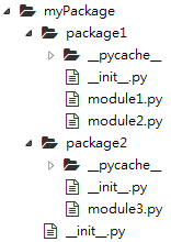
記得此時要將module2內的from package1 import module1 as m1修改為from myPackage.package1 import module1 as m1。接下來的用法差不多,以下的寫法都可以:
from myPackage.package1 import module2 as m2 poly = m2.polygon(0, 30) print(poly)或是
import myPackage.package2.module3 as m3 m3.fun3_1()不過以下的寫法就不行:
from myPackage import package2.module3 as m3 m3.fun3_1()都是package,不要把它們拆開來寫就行了。再進一步,如果在module3建立一個class名為squre且其繼承module2中的polygon,那麼該如何寫呢?
from myPackage.package1 import module2 as m2 class square(m2.polygon): def area(self): return self.a*self.b def __repr__(self): return f"A square with a={self.a}, b={self.b}, area={self.area()}"接著執行以下指令:
from myPackage.package2 import module3 as m3 s = m3.square(4, 10, 20) print(s)結果如下:
A square with a=10, b=20, area=200
-
Talk54_1.py
myPackage.zip
- 將module或package跟主程式放在同一個資料夾,在package內增加一個__init__.py的檔案
- Import的語法:
- 僅有module:import module
- 有package: from package import module、import package.module
- 有package與subpackage: from package.subpackage import module、import package.subpackage.module
Recap
Python亂談
其他
第五十五話、檔案
當我們有外部資料在一個檔案內,或是要將資料寫入到其他檔案中,我們需要開啟跟一個檔案的資料流連結,然後進行資料的讀取或寫入,使用的關鍵字是open。首先先看一下它的解釋:help(open)
open(file, mode='r', buffering=-1, encoding=None, errors=None, newline=None, closefd=True, opener=None)
其中有個參數mode='r',內定值是r,其他的值為:
========= ===============================================================
Character Meaning
--------- ---------------------------------------------------------------
'r' open for reading (default)
'w' open for writing, truncating the file first
'x' create a new file and open it for writing
'a' open for writing, appending to the end of the file if it exists
'b' binary mode
't' text mode (default)
'+' open a disk file for updating (reading and writing)
'U' universal newline mode (deprecated)
========= ===============================================================
可以看出如果要讀檔案,可以使用r (default)、r+、w+,若是要寫入檔案,可以使用w、x、a、r+、w+。b是指binary格式的檔案,我們若不指定,便是文字模式的t。搞定,來試個例子寫入檔案、例如:
f = open('temp.txt', 'w') f.write("writing something") f.close()首先當我們使用open時,根據傳入參數定義,第一個是檔案名,第二個是mode,其他都是預設值。而此函數傳回一個TextIOWrapper物件,在此命名為f。當我們查詢TextIOWrapper物件方法(help(f)),可以看到write()這個方法,讓我們可以將字串寫入檔案內。最後要使用close()方法來關閉IO物件,如果沒有close,那會一直保持開啟,你若打開寫入檔案(temp.txt),你會看到空白內容,有了close後,內容才會顯示。接著將w換成w+或r+試試看:
f = open('temp.txt', 'w+') for i in range(10,20): f.write(f"{i} \n") f.close()原則上都是相同的,不同處是使用w或w+時,若是檔案不存在則根據輸入的檔名建立新檔案,但若是使用r+時,檔案(使用temp1.txt)不存在則傳回錯誤。
(FileNotFoundError: [Errno 2] No such file or directory: 'temp1.txt')
而若是使用x則相反操作,先檢查該檔案是否存在,若不存在則建立新檔案然後寫入,若是已存在則傳回錯誤。
(FileExistsError: [Errno 17] File exists: 'temp.txt')
f = open('temp1.txt', 'x') for i in range(100,120): f.write(f"{i} \n") f.close()那麼若是使用a呢?原則上a就是append,相當熟悉的一個字,就是附加在檔案原資料後面。
f = open('temp.txt', 'a') for i in range(100,120): f.write(f"{i} \n") f.close()那如果檔案也是不存在呢?也沒問題,會自動建立新檔案。接下來若是要讀取檔案呢?首先直接使用預設的r。
f = open('temp.txt') print(f.read()) f.close()當使用read()這個方法(使用初始參數)或是參數size為負數(e.g. size=-1),會讀取所有內容。此方法可以輸入參數來強調要讀取的字元數,例如如果使用read(16),那麼一次讀取16字元。
f = open('temp.txt') print(f.read(16)) print(f.read(16)) f.close()不過有時候我們可能會想一次讀一行,此時使用readline()這個方法,順便試一下r+。如下:
f = open('temp10.txt', 'r+') while True: line = f.readline() if line != '': print(line, end='') else: break f.close()使用f.readline()來一次讀取一行。當讀到的內容為’’,則表示到檔案的最末端了(end of file),此時結束。當檔案不存在時,而r及r+會回傳錯誤(FileNotFoundError: [Errno 2] No such file or directory: 'temp9.txt')。不過一般來說我們可以直接使用for loop來進行比較容易,如下:
f = open('temp.txt', 'r+') for line in f: print(line, end='') f.close()end=''只是避免每次讀一行都換行兩次。那麼若使用w+來讀取怎麼辦?w+是比較特殊的,當使用w+時,檔案若是不存在,則會建立一個新檔案,檔案若是已存在,那麼首先會將內容清空,也就是此時也讀不到東西,若有寫入資訊後,可跳到資料流開頭開始讀。例如:
f = open('temp.txt', 'w+') for i in range(10): f.write(f"{i}\n") f.seek(0) for line in f: print(line) f.close()當使用w+時,因為檔案已存在,所以內容會先被清空,然後使用f.write()寫入資料。f.seek(0)這個指令的內容如下:
help(f.seek)可見使用0回到開頭,然後再使用for line in f:來讀取,一次一行。
每次使用open()時,都要記得使用close(),不然會出錯。不過總是要記得有點麻煩,所以Python提供另一個語法可以解決這個問題,使用with關鍵字,舉例如下:
with open('temp.txt', 'r+') as f: for i in range(200, 220): f.write(f"{i}\n")這個寫法可以讓我們無須close(),自動達成,酷吧。此外,如果我們直接使用以下語法,會出現怎樣的狀況?
for line in open('temp.txt','r'): print(line, end='')這樣直接讀取看起來結果是一樣的,不過不太正統,好像在某些作業環境下有可能出錯,所以最好還是這樣寫:
with open('temp.txt','r') as f: for line in f: print(line, end='')這樣就沒有問題了。最後做個練習,將temp.txt的內容讀出來,然後寫到另一個檔案temp10.txt內。
with open('temp.txt','r+') as f: content = f.read() with open('temp10.txt', 'w') as f: f.write(content)唔,用這樣複製檔案內容好像太簡單了。再用另一個寫法:
content = open('temp.txt','r').read() f = open('temp11.txt','w') f.write(content) f.close()嗯,用with比較好。(・_・;)
-
Talk55_1.py
temp10.txt
- 使用open()建立檔案連結,記得使用close()
- 使用with關鍵字不需要使用close()
- 寫入檔案時mode參數使用w、x、a、r+、w+,讀取檔案時mode參數使用r (default)、r+、w+
Recap
第五十六話、遞迴函數
又回頭來談函數,不愧是亂談 (#^.^#)。在之前談函數時提到若是兩個函數互相呼叫,可能會變成類似無窮迴圈一般無窮無盡,必須要設定一個停止條件。遞迴函數跟這情況有點類似,不過是函數自己呼叫自己。首先先來看個例子:0! = 1 n! = n*(n-2)*(n-2)*...*2*1這是階乘的定義,我們可以很輕易地建立一個函數來求取n!。
def fac(n:int): f = 1 for i in range(1,n+1): f = f*i return f事實上我們了解n!就是n*(n-1)!,(n-1)!就是n-1*(n-2)!,依此類推。所以我們也可以這樣寫:
def fac2(n:int): if n <= 1: return 1 # 基礎條件 else: return n*fac2(n-1) # 遞迴公式這個寫法相當口語化,只要有基礎的停止條件,然後給定遞迴公式即可。那麼它的內涵是甚麼呢?
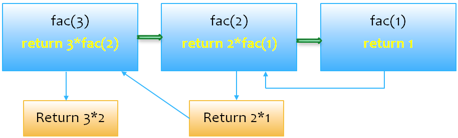
如上圖所示,當要計算fac(3)時,會先呼叫fac(2),要計算fac(2)時,又呼叫了fac(1),因為fac(1)=1(基礎條件),所以將值回傳到fac(2),得到fac(2)=2*1=2,再將fac(2)回傳到fac(3)=3*fac(2)=3*2=6。甚至a*b都可以拆解為a+a*(b-1),函數做法如下:
def mul(a,b): if b == 1: return a else: return a + mul(a,(b-1))用這個方式把相乘變成連加,也就是a*b = a+a+a+…+a(b次)。不過這就讓我們納悶了,這樣寫程式有比較省事嗎?直接相乘不是就好了嗎?沒錯,遞迴(recursive)並不見得在每個例子中都完勝迭代(iterative),總是互有優劣。在討論遞迴時,難免要提到最著名的費氏級數(Fibonacci Sequence),相傳一開始的題目是由數學家Fibonacci提出,是說一對兔子每個月會生下另一對兔子,新生的兔子需要兩個月後才能開始加入生育,且兔子永不死亡,假設一開始有一對兔子,那麼每個月會有多少對兔子?
一開始有一對新生兔子,一個月後因為尚未長大,所以還是一對兔子,因此一開始兩個月的數字為1,1。第三個月初生下一對兔子,所以總共為2對,數列變成1,1,2。第四個月初原先的成兔又生下一對兔子,再加上原先尚未成長完成的兔子,總共有三對,數列變成1,1,2,3。之後一個月,最先出生的一對兔子成長為成兔並生下一對兔子,加上原先的成兔也生下一對兔子,所以總共增加2對兔子,加上原本的3對兔子,總共有5對兔子,數列變成1,1,2,3,5。依此類推,可以發現每個月的兔子總對數剛好是前面兩個月的兔子個數相加。這個數列稱之為費氏數列。一般表示如下:
0,1,1,2,3,5,8,13,……那其遞迴程式要怎麼寫呢?如下:
def fib(n:int): if n==0: return 0 # 基礎條件 elif n==1: return 1 # 基礎條件 else: return fib(n-1)+fib(n-2) # 遞迴公式測試一下:
for i in range(10): print(fib(i))嗯哼,符合期待。那若是不用遞迴的方式怎麼寫?
def fib2(n:int): if n==0: return 0 elif n==1: return 1 else: a,b=0,1 for i in range(n): a, b = b, a+b return a一樣測試會得到相同的結果。雖然這樣的寫法比之遞迴較不直覺,但是執行速度應該會快一些,遞迴程式每一次需要呼叫自己兩次,反而沒甚麼效率。這裡順便提一下中間的a,b=b,a+b這行指令,本來這行應該是要這樣寫:
a, b = 3, 5 c = a + b a = b b = c print(a) print(b)但是Python讓我們可以使用a,b=b,a+b這樣的語法來簡化過程。又好比我們有a跟b兩個變數,如果要讓其值對調(稱為swap)要怎麼寫?本來應該要這樣:
temp = a a = b b = temp print(a) print(b)不過我們可以很簡單的使用a, b = b, a即可(^o^)。
再做個遞迴的練習,假設有兩數,要怎麼找到其最大公因數?這個問題就算不會遞迴也可以很輕鬆地做到,如下:
def gcd(a,b): g = 1 if a < b: upper = a else: upper = b for i in range(2, upper+1): if a%i==0 and b%i==0: g = i return g先找到比較小的數,然後一個數一個數的除除看,只要可以整除兩數的最大數就是最大公因數了。不過這個做法在數字比較大的時候,會需要計算很多次,當然有人想說反正是電腦在算,我又不累,不過如果我們可以讓其計算量減少,效率可以提高不少。所以小時候學過輾轉相除法,比一個數一個數來得經濟許多,但是我們卻不知道輾轉相除法要除幾次才會得到答案,此時用遞迴方式來編碼正好。
def gcd2(a,b): """ Recursive method to obtain g.c.d. """ if b%a == 0: return a else: return gcd2(b%a, a)這個方法得到最大公因數,需要計算的次數就少許多了。最後請自己試一下怎麼印出一個正整數的二進位制表示,做法參考如下:
def binary(x): if x == 0: return '0' else: return binary(x//2)+str(x%2)
Talk56_1.py
-
Recap
- Recursive函數就是會持續呼叫自己的函數,需設計停止條件讓它停止
第五十七話、generators
在我們使用for loop時,會一次一個的走遍(traverse)整個iterable的物件,那是因為iterable物件都有一個方法稱為__iter__(),它會傳回一個iterator物件,而這個物件有一個方法稱為__next__(),它會一直的指向下一個元件,直到我們歷遍所有元件。也就是說我們可以這樣做:lista = [1,2,3] itera = iter(lista) print(next(itera)) print(next(itera)) print(next(itera)) print(next(itera))當每一次呼叫next()後,便會傳回下一個元件,待到next指向空時,傳回StopIteration物件,此物件註明iterator.__next__()的尾端。使用這個形式,我們可以定義自己的iterable物件,例如:
class myIterable(object): def __init__(self, start, stop, pace = 1): self.start = start self.stop = stop self.pace = pace def __iter__(self): return self def __next__(self): if self.start < self.stop: x = self.start self.start += self.pace return x else: raise StopIteration這個class內包含__iter__()與__next__()兩個方法,所以是iterable物件。在__next__()方法內,每次傳回目前值,然後加上步幅,等待下次呼叫,直到超過長度為止,原則上跟range()的概念相同。現在我們可以有自訂的range()了,那generator又到底是甚麼呢?其實是要做類似的事情,不過generator使用關鍵字yield,讓我們不需要定義__next__()方法就可以建立iterator,而且此方法號稱可以減少記憶體使用率,現在看個例子:
def myGenerator(n): """ A generator that increase 1 each time """ i = 0 while i<n: yield i i+=1理論上我們使用while i
def myRange(*arg): """ Function myRange(start, stop , pace) Same to range() """ if len(arg) == 1: start = 0 stop = arg[0] pace = 1 elif len(arg) == 2: start = arg[0] stop = arg[1] pace = 1 elif len(arg) == 3: start = arg[0] stop = arg[1] pace = arg[2] else: raise TypeError('Number arguments error.') while start < stop: yield start start += pace還記得上一話提到的fibonacci sequence,現在利用這個方式來設計一個class,每次傳回下一個fibonacci number,如下:
class Fibonacci(object): def __init__(self, n): self.n = n self.a = 0 self.b = 1 def __iter__(self): i = 0 while i <= self.n: yield self.a self.a, self.b = self.b, self.a+self.b i+=1當呼叫iter(),傳回一個iterator(使用generator達到此目的)。執行結果如下:
for i in Fibonacci(5): print(i)再看一個例子,利用之前的myRange(),可以設計如下的函數:
def square(a,b,c): for i in myRange(a,b,c): yield i**2 def squareList(a,b,c): slist = [] for s in square(a,b,c): slist.append(s) return slist在square()內使用myRange()且函數square()也是一個generator,一樣傳回一個iterator,然後在squareList()內使用square(),測試結果如下:
print(squareList(2,20,2))我想各位現在對於iterator與generator應該都沒有問題了。還記得之前我們談過的list comprehensions?
[x for x in range(5)]我相信各位一定記憶猶深,提這做甚麼呢?原來也可以用類似的方法製作generator,叫做Generator Expressions,只要把中括號換成小括號即可。例如:
r = (x for x in range(3)) print(type(r))此時r是一個generator,所以我們可以做類似如下的事情:
for i in r: print(i)或是
r = (x for x in range(3)) print(list(r))甚至
r = (x for x in range(3)) print(sum(r))都是因為r就是一個generator。好吧,再試一個我們的老朋友,求質數的generator,一行搞定。
p = lambda n : (x for x in range(2, n) if all([x%y!=0 for y in range(2,x)]))測試結果如下:
for i in p(10): print(i)最後再看一個讀取多個檔案的應用。假設我們有兩個檔案內容如下:
| file1.txt | file2.txt |
| one little two little three little indians … | The itsy bitsy spider Went up the water spout Down came the rain and Washed the spider out … |
files = ["file1.txt", "file2.txt"] def readMFiles(filenames): for file in filenames: with open(file) as f: for line in f: if "indian" in line or "spider" in line: print(line)毫無疑問的,當我們呼叫readMFiles(files),會顯示出所有符合條件的句子。不過這個函數的層數蠻多的(Nested),雖然我們了解內涵,不過根據Python之禪(Flat is better than nested.),這並不是最好的做法。若是使用generator的方式來寫,便可拆成幾個函數如下:
def readFiles(filenames): """ 讀取所有檔案內的所有句子,傳回generator """ for file in filenames: with open(file) as f: for line in f: yield line def gen(lines): """ 在所有傳入句子中萃取所有符合某條件的句子 """ return (line for line in lines if "indian" in line or "spider" in line) def printResults(filenames): lines = readFiles(filenames) lineGens = gen(lines) for line in lineGens: print(line)好吧,看起來好像變長了不少,不過拆成幾個函數靈活度跟可讀性都會變高了。例如若是可以把選取句子的條件變成參數,只要在gen()內做點修正即可,邏輯容易清楚。
-
Talk57_1.py
file1.txt
file2.txt
- 了解iterator與generator,可使用yield關鍵字產生generator
- 可以使用Generator Expressions來產生generator
Recap
第五十八話、時間
在很多的時機裡,需要跟時間打交道。所謂跟時間打交道指的是我們可能會需要日期、時分與時間差。在此我們介紹datetime這個模組,在此模組中包含以下幾種主要的class:- Date : 主操縱日期(Month, day, year)
- Time: 操縱時間(Hour, minute, second, microsecond)
- Datetime: 時間跟日期合併(Month, day, year, hour, second, microsecond)
- Timedelta: 操作一段日期內的時間
- Tzinfo: 跟時區有關的操作
- Timezone: 3.2版後新加入的操作時區之物件
from datetime import date print(date.today())today()是date物件裡面的一個方法,傳回今天的日期。在這個函數包含三個參數(day、month、year),我們可以根據以下方式取得參數值:
date.today().day date.today().month date.today().year如果要得到星期幾呢?在today()內有一個方法叫做weekday(),會傳回星期的編號:
date.today().weekday()傳回2,不過看了一下日歷,咦,今天是星期三,嗯,原來他的儲存方式自星期一到星期日對應0到6,所以跟我們認識的星期幾要再加1。我們可以使用這樣的方式來得到星期幾的表示:
weekdays = ["monday","tuesday","wednesday","thursday","friday","saturday","sunday"] weekdays[date.today().weekday()]之前提到這個模組中有5個物件,其中date跟datetime都可以操作日期,所以現在我們同時試一下datetime裡面的目前時間,使用的是now()這個方法。
from datetime import datetime as dtime print(dtime.now())now()會傳回一個datetime物件包含目前的日期時間。我們可以使用dtime裡面的date()跟time()兩個方法來分別得到date跟time物件,這兩個方法需要傳入一個datetime物件作為參數,剛好我們可使用now()來產生這樣的物件。
datenow = dtime.date(dtime.now()) timenow = dtime.time(dtime.now()) print(f"Date: {datenow}", Time: {timenow})這樣可以將日期時間分拆開來。
now()得到的日期時間格式是這樣2019-01-09 19:17:54.928611,如果我們想要其他格式的表示要怎麼做?在date物件中有一個方法strftime()可以來格式化時間字串,datetime也繼承了這個方法,我們先看一個例子:
now = dtime.now() print(now.strftime("%D"))跟之前一樣要印出now的時間,只是使用strftime()這個方法來改變顯示格式,這個方法需要我們輸入想要的格式字串,當我們輸入%D這個符號,表示要顯示日期,所以會出現01/09/19。也就是說只要我們輸入不同格式就會出現不同的時間顯示,那我們怎麼知道有哪些格式?原則上我們可以使用以下的符號:
| 符號 | 說明 | 舉例 |
| %a | 星期縮寫 | Sun, Mon, …, Sat (en_US); |
| %A | 星期 | Sunday, Monday, …, Saturday |
| %w | 星期編號、0是星期日、6是星期六 | 0, 1, …, 6 |
| %d | 日的編號 | 01, 02, …, 31 |
| %b | 月的縮寫 | Jan, Feb, …, Dec (en_US); |
| %B | 月的全名 | January, February, …, December |
| %m | 月的編號 | 01, 02, …, 12 |
| %y | 年的二碼編號 | 00, 01, …, 99 |
| %Y | 年的四碼編號 | 0001,…, 2018, 2019, …, 9999 |
| %H | 小時(24-時制) | 00, 01, …, 23 |
| %I | 小時(12-時制) | 01, 02, …, 12 |
| %p | 上下午(AM or PM.) | AM, PM (en_US); |
| %M | 分 | 00, 01, …, 59 |
| %S | 秒 | 00, 01, …, 59 |
| %f | 毫秒 | 000000, 000001, …, 999999 |
| %Z | 時區 | (empty), UTC, EST, CST |
| %j | 年中的日 | 001, 002, …, 366 |
| %U | 年中的星期(星期日為星期的第一日) ,編號0表示第一個星期日之前的星期 | 00, 01, …, 53 |
| %W | 年中的星期(星期一為星期的第一日) ,編號0表示第一個星期一之前的星期 | 00, 01, …, 53 |
| %c | 當地合適的日期時間顯示 | Tue Aug 16 21:30:00 1988 |
| %x | 當地合適的日期顯示 | 08/16/1988 (en_US); |
| %X | 當地合適的時間顯示 | 21:30:00 (en_US); |
print(now.strftime("%c")) print(now.strftime("%d/%b/%Y %X")) print(now.strftime("%Y-%B-%d %A %I:%M:%S %p"))看來我們可以自己隨意搭配,喜歡怎樣的格式就怎麼穿搭。接下來我們再來了解一下timedelta這個物件。首先還是要import,這裡使用以下格式:
from datetime import timedelta as tdelta接著看以下例子:
delta = tdelta(days = 10, minutes = 2, seconds = 30) print(delta) print(tdelta(days = 10, minutes = 2, seconds = 30))這行指令顯示了10 days, 0:02:30,timedelta物件可以讓我們輸入一個時間,但是這有甚麼用?看一下下一步:
print(f"today is {dtime.now()+delta}")顯示了today is: 2019-01-19 20:34:17.552842,這個有點意思了,兩個時間可以加起來。原來timedelta是一個時間間隔,可以讓我們計算時間差的,而兩個時間的差距(+或-)會傳回timedelta物件。假設有一個重要的日子是一月23日,我們想要知道從現在到那天還差幾天,可以寫這樣:
someday = date(2019, 1, 23) delta = someday - date.today() print(f"Days to 1/23 is {delta}") # Days to 1/23 is 14 days, 0:00:00若是使用datetime物件也可以,記得相減也要兩個是相同物件:
sometime = dtime(2019, 1, 23, 12, 30, 30) delta = sometime - dtime.now() print(f"Time to 1/23 noon is {delta}") # Time to 1/23 noon is 13 days, 15:46:52.263366如此我們可以算出兩個時間的差,或是計算一個時間跟一個時間差(timedelta)的和。這在很多要計算時間的程式中可以應用,例如不停地計算還有幾天要考試或是周年慶等等,甚或是計算一個程式的執行時間都可以。例如我們回顧到第58話的例子,在最後修改成如下:
if __name__=="__main__": start = datetime.datetime.now() nnodes = 200 # number of nodes in the problem iteration = 2000 # number of iterations route = Route(nnodes) route.newRoute(iteration) print(f"minList = {route.minList} \nminLength = {route.minLength}") route.plotFigure() stop = datetime.datetime.now() print(f"Time used: {stop - start}")藍色框是用來計算執行時間用的,紅色框裡的數據變大是讓我們比較有感覺一點,因為原來都是設定20連1秒都沒有就結束了。
-
Talk58_1.py
- 使用時間物件前先import datetime模組
- 時間可以用strftime()方法來顯示不同格式
- 兩個時間差可以直接計算且會傳回timedelta物件
Recap
第五十九話、還有時間
在Python中還有另一個跟時間有關的模組稱為time,這個模組主要是使用實數(秒)來記錄經過的時間,主要的時間標準為1970年1月1日0時,所以如果我們import time,便可以使用time()這個方法來得到自那日起到目今所經過的所有秒數,例如:import time print(time.time())得到的結果是1547097674.7630448,換算了一下當然是沒錯(錯了就糟了),不過得到秒數對於計算可能容易,對於顯示內容就不好理解了。所以顯然有方式能讓我們得到其他顯示結果,顯示方式主要是以9個數字形成的time tuple來表示,根據help的內容,數字的代表內容如下:
- year (including century, e.g. 1998)
- month (1-12)
- day (1-31)
- hours (0-23)
- minutes (0-59)
- seconds (0-59)
- weekday (0-6, Monday is 0)
- Julian day (day in the year, 1-366)
- DST (Daylight Savings Time) flag (-1, 0 or 1)
time.localtime()可以看出來localtime()傳回一個名為struct_time的物件,內容包含上述的9個數據。struct_time是這個模組的主要class,模組內的函數如gmtime(), localtime(), and strptime()都會回傳struct_time物件,並可被asctime(), mktime() and strftime()這些函數接受。Class內定義了相關的參數,所以我們可以分別得到參數內容,例如:
k = time.localtime() k.tm_year k.tm_hourtime也包含strftime()這個函數,可以讓我們得到跟datetime一樣的時間格式,如果沒有傳入參數(struct_time物件),那就會自動變成顯示localtime(),也就是目前時間,例如:
print(time.strftime("%Y-%B-%d %A %I:%M:%S %p"))顯示結果為2019-January-10 Thursday 01:43:58 PM,與之前一話的顯示格式完全相同。
因為time這個模組中最主要的數據是秒數,只要得到秒數,就可以換算時間,得到時間,也可以換回秒數,相關的函數先介紹ctime()。例如:
period = 31536000*50 # 365*24*60*60*50 theTime = time.ctime(period) print(theTime)此方法傳回一個字串,顯示為Fri Dec 20 08:00:00 2019,也就是只要我們傳入一個秒數進入ctime(),他就會幫我們計算自時間標準(1970/1/1)開始經過這些秒數後的時間,上例我們輸入50年的秒數。也可以使用asctime()這個函數,此函數直接輸入9個數字的time tuple來取得時間點,例如:
time.asctime((2019, 1, 10, 10, 33, 30, 0, 0, 0))不過事實上上例這個時間是星期四,但是因為我們輸入星期一,所以便顯示星期一,也就是說這並不是一個正確時間,不過因為只是星期錯誤,比較不影響其他內容。如果我們不需要特別的格式,也可以快速的使用這個函數顯示時間:
time.asctime(time.localtime())原則上time.localtime()可以省略,因為localtime本來就是asctime()的輸入參數預設值。反過來說,如果給定某個時間然後想得到秒數,那就使用mktime(),需要傳入時間參數。例如:
s = time.mktime(time.struct_time((2019, 1, 10, 10, 33, 30, 0, 0, 0))) print(s)或
s = time.mktime((2019, 1, 10, 10, 33, 30, 0, 0, 0)) print(s)這可以得到自標準時間到此時間所經過的秒數。因此以下兩者應會得到相同結果:
print(time.mktime(time.localtime())) # 1547101924.0 print(time.time()) # 1547101924.029089因為有顯示出來的時間差,還是差了一些些= =”。
若有秒數,傳入ctime()可以得到時間字串,但若要得到struct_time物件,就要用到gmtime()這個函數,例如:
st = time.gmtime(s) print(st)有了這個物件,又可以使用time.asctime(st)來得到時間字串。那若是要將字串轉回time tuple,則使用strptime("%a %b %d %H:%M:%S %Y"),也就是逆轉strftime()的輸出結果,例如:
tt = time.strptime("Thu Jan 10 14:30:30 2019") print(tt)到這裡先歸納一下:
- time():取得到目前的秒數
- mktime (time tuple):給time tuple傳回秒數
- ctime (秒數):傳回給定秒數計算後之字串
- asctime (time tuple):給time tuple傳回時間字串
- strftime(time tuple):格式化time tuple(預設為目前時間)的時間
- strptime(time tuple):將格式化時間字串轉回time tuple
- localtime ():傳回目前時間物件(struct_time)
- gmtime (秒數):傳回給定秒數計算後之時間物件(struct_time)
start = time.time() time.sleep(3) stop = time.time() print(stop-start)停止一下這個執行緒(thread)到底有甚麼用?想像一下我們可能要設計一個時鐘,一個倒數計時的裝置(跨年或定時炸彈),都需要讓時間有所延遲,此時sleep()就可能有用處了,例如:
for i in range(10, -1, -1): print(i) time.sleep(1)倒數10秒。
之前提到若要計算某程序的執行時間,可以使用前後時間相減來達成,不過如果只是想要知道某小段程式(snippet)敘述的執行時間,還有另一個選擇就是使用timeit這個模組。用法如下例:
timeit.timeit("sum(list(range(100)))")只要將要執行的程式片段做成字串,傳入timeit.timeit()方法內,即可得到執行所需時間。不過這個單位是甚麼?秒嗎?怎麼會需要這麼久呢?再仔細看一下help:
help(timeit.timeit)原來有一個參數number的預設值是1000000,也就是跑了1000000次需要的時間。用剛才學的time模組測試一下:
import time start = time.time() for _ in range(1000000): k = sum(list(range(100))) stop = time.time() print(f"{stop}-{start} = {stop-start}")大概差了個0.1秒上下,因為這段程式碼做了些額外的事情,所以應該是正確的。如果我們把要測試的內容寫成函數如下:
def test(x): return sum(list(range(x)))要測試這個函數,需要使用setup參數,做法如下:
print(timeit.timeit("test(100)", setup = 'from __main__ import test'))假如牽扯到不只一個函數,那就使用globals參數,例如:
import math def t1(x): return sum(list(range(x))) def t2(x): return math.sqrt(x) def t3(x): return math.log(math.pi/x) print(timeit.timeit("[x(10) for x in (t1,t2,t3)]", globals=globals()))globals()這個函數是built-in function,會回傳目前所有的全域變數。
如果我們想要重複的執行某一個timeit.timeit(),看看每次有沒有太多差別,可以直接使用repeat()這個函數:
print(timeit.repeat("[x(10) for x in (t1,t2,t3)]", globals=globals(), repeat = 5))內定是執行3次,若要改變次數,可以使用參數repeat =5來修改為執行5次,結果會儲存在一個list內。
-
Talk59_1.py
Talk59_2.py
- import time模組之後可以使用相關方法來取得秒數,取得時間字串,或是取得時間物件(或time tuple)
- 使用timeit模組可以計算某一個片段的程式碼之執行時間
Recap
第六十話、讓我看一下日曆選個好日子
既然時間的模組都講了,再來看一個日曆的模組,calendar。首先當然是先把它import進來,看一下其中包含的物件,計有Calendar、TextCalendar、HTMLCalendar、LocaleTextCalendar、LocaleHTMLCalendar等,其中有HTML的跟網頁設計有關,Calendar物件不提供格式,僅提供資料給子類別(subclasses)。有Locale表示可以得到當地的名稱。看來選擇不多,來試一下TextCalendar,做法如下:import calendar #取得一個TextCalendar的物件 tc = calendar.TextCalendar() # 使用formatmoonth()傳回某一個月的calendar字串 tcstr = tc.formatmonth(2019, 1) # 印出該月的月曆 print(tcstr)其中tc是TextCalendar的物件,formatmonth()是該物件的方法,參數是某年某月,傳回的字串如下:
相當帥( ͡° ͜ʖ ͡°)。相關的方法有formatyear:
yearstr = tc.formatyear(2019) print(yearstr)可以印出整年的月曆。若是僅要印出月曆,也可以使用prmonth()或pryear()等方法。
tc.prmonth(2019,1) tc.pryear(2019)如果僅是要印出某月的月曆,也可以這樣:
print(calendar.month(2019,1))仔細觀察所有的月曆,第一天都是星期一,如果想換成星期日呢?那在宣告物件的時候需要輸入第一天的參數,可以使用calendar.SUNDAY或6代表星期天。如下:
tc = calendar.TextCalendar(calendar.SUNDAY) #tc = calendar.TextCalendar(6) print(tc.formatmonth(2019, 1))現在可以看到月曆的第一天是星期天了,其他依此類推,本來的預設值是calendar.MONDAY(0),若要使用譬如星期三當作第一天,就給參數calenday.WEDNESDAY或2即可。順便用以下的code來測試一下HTMLCalendar:
htmltc = calendar.HTMLCalendar() print(htmltc.formatmonth(2019,1))語法原則上完全相同,印出來後會得到一堆HTML的程式片段,如果把它們貼到一個文字檔儲存成.html的檔案,然後使用網頁瀏覽器開啟的話,你將會看到一個有月曆的網頁。
接下來我們使用itermonthdays()這個方法來取得月曆中的所有日,並使用for loop來走過一遍。
tc = calendar.TextCalendar(calendar.SUNDAY) for i in tc.itermonthdays(2019, 1): print(i)你會看到一開始是0,後面才出現1到31然後又是0,0表示在這個月歷中不是這個月份的日子,因為有5周,所有總共會印出35個數字。其他的相關方法有
for i in tc.itermonthdates(2019, 1): print(i) for i in tc.itermonthdays2(2019, 1): print(i) for i in tc.iterweekdays(): print(i)Itermonthdates()會印出2019-01-10這種形式、itermonthdays2()會印出tuple例如(10, 3),3表示Thursday、而iterweekdays()則印出0-6表示星期幾。此外,以下方式會印出星期與月份的名稱。
for day in calendar.day_name: print(day) for month in calendar.month_name: print(month)在Python3.7版中新加入itermonthdays3()與itermonthdays4()方法,若你的Python版本高於該版本可以試試看。再者,calendar.monthcalendar()方法會傳回該月日曆的二維陣列,如下:
mc = calendar.monthcalendar(2019, 1) print(mc)好了,現在我們可以嘗試印出2019年每個月的第一個星期日是幾號:
for month in range(1,13): mc = calendar.monthcalendar(2019, month) m = calendar.month_name[month] sunday = mc[0][6] print(f"{m}的第一個星期日是{sunday}號")因為calendar.monthcalendar()的排列方式是星期一在第一天,所以第一個星期日都會在第一周,若是題目是要印出第一個星期一就要判斷第一周的第一天是不是為0,0的話表示星期一在第二周。
-
Talk60_1.py
- TextCalendar物件可以使用formatmonth()方法來得到月曆字串
- HTMLCalendar物件使用formatmonth()方法得到的是HTML的月曆字串
- 使用itermonthdays()方法來traverse月曆中的每一日
- 使用calendar.monthcalendar()方法來傳回該月日曆的二維陣列
Recap
第六十一話、不知名的老生常談
想不出這一話要給甚麼名字,總之要熟悉一個東西,只有一個最好的笨方法就是多練習,這次來試試看這個題目。首先給定一個檔案名為T61_nodes.txt,其中包含了100個資料,每一筆資料有三個數字分別為點的編號(0-99)、x座標(0-100)、y座標(0-100),中間用逗點分隔,譬如0, 19, 100。點的分布如下圖: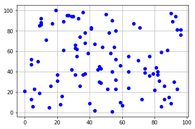
好吧,事實上檔案與圖的資料也是使用之前學過的語法隨機產生的,請參考Talk61_1.py。再次強調繪圖的部分之後再提。先假設這些點都是一些客戶的位置,現在好比說要找一個好地方開一間咖啡廳,這個位置要使得所有客戶到咖啡廳的總距離最短。這樣的題目叫做選址問題,這裡不討論,只假定最好的位置是在重心(其實並不是,若想知道更多可以查詢weber problem或facility location problem或p-median problem)。重心的公式是
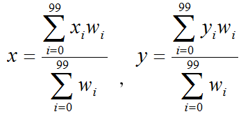
好像很複雜,因為這裡的客戶權重相同,也就是沒有VIP客戶,所以 都等於1,因此分母都是100,而分子就是所有x(或y)座標的和,我們可以得到(48.39,50.79)這個座標做為開咖啡廳的位置。靠近(50,50),對於在100x100的平面上產生的隨機點來說,是合理的數據。不過這不是這裡要求的(~_~;),我們的目標是如果要在這些客戶中開啟三間咖啡廳的話,要在哪三個位置?當然還是想要大家距離咖啡廳近一點,這樣生意才會好。這裡採用k-means的方法,這是甚麼方法?作法是先隨意地找三個地點,然後將這100個客戶分成三群,分群的規則就是看距離哪個地點最近就屬於哪一群。現在隨意地分了三群客戶,接下來根據每一群的客戶位置找到該群的重心,這三個重心現在是新的開咖啡廳的地點。接下來就是重複的步驟,根據這三個新地點再將客戶分群,再根據各群找出新重心,再分群再找重心,重複幾次之後,應該就不會有太大的變化,此時我們就找到了三個開咖啡廳的位置了。
好了,了解了題目就可以開始coding了(Talk61_2.py)。首先我們想到應該先把檔案內的資料讀進來然後才能操作,沒錯,檔案內有100個點的資料,讀進來之後可以放在一個容器(e.g. list)內,不過要描述一個點,應該先有個class會比較好操作。這個之前做過了,先來個點的class如下:
class Node(object): """ 一個點的class """ def __init__(self, nodeid, x, y, group = -1): self.nodeid = nodeid self.x = x self.y = y self.group = group def __repr__(self): return f"{self.nodeid}, {self.x}, {self.y}, {self.group}" __str__ = __repr__跟之前的很類似,不過多了個參數group。這是因為根據上述的演算方式,每個點(客戶)都需要屬於某一個群組(咖啡廳),所以特別設計這個參數來記錄。接下來就可以把資料讀進來,然後將每行資料轉換成一個node物件,放在一個list內,做法如下:
nodes = [] # ============================================================================= # 讀取檔案內資料 # ============================================================================= with open("T61_nodes.txt", 'r') as f: for line in f: record = line.split(',') nid = int(record[0]) x = int(record[1]) y = int(record[2]) nodes.append(Node(nid, x, y))嗯,這也不難。現在整個資料都準備好了,現在要隨機產生三個點作為咖啡廳,三個點還是node的物件,為了不要跟客戶的點搞混,三個點的編號定為1001、1002、與1003。位置就隨機產生,所以要記得加上import random as rd。
有了初始的三個位置後,馬上就將客戶分組,這裡將其分割為兩個函數,因為分組跟距離有關,所以第一個函數是計算距離的函數,這個之前練習過。
def distance(n1:Node, n2:Node)->float: return ((n1.x-n2.x)**2+(n1.y-n2.y)**2)**0.5第二個函數是幫每個客戶找最近咖啡廳的函數,必須計算到每個咖啡廳的距離然後取最小,找到之後就直接把nodes裡面物件參數(group)修改掉,如下:
def nearestCoffee(n:Node, shops:list)->int: """ 尋找最近點 """ for i, s in enumerate(shops): dis = distance(n, s) if i==0: shortest = dis shortestid = s.nodeid else: if dis < shortest: shortest = dis shortestid = s.nodeid nodes[n.nodeid].group = shortestid return shortestid之後只要把每個點都應用到nearestCoffee()即可。如下:
for i in nodes: nearestCoffee(i, coffeeshops)現在觀察nodes裡面的點,group的值就重新指派了。有了這些group的值,就可以根據每一個group找到新的重心,再寫成一個函數:
def center(g): """ 計算重心座標 """ sumx = 0 sumy = 0 w = 0 for n in nodes: if n.group == g: sumx += n.x sumy += n.y w += 1 return (sumx/w, sumy/w)計算屬於此group的所有點之x與y之和,然後除以個數(w)即可。其實這裡有可能出現一個錯誤,那就是w可能為0,使得分母為0。為何會出現這個錯誤呢?那是因為可能有兩個候選點距離太近又靠近邊緣,造成其中某一個分群裡面沒有客戶。所以我們可以做些彌補,例如在w等於0的情況下,傳回特定值,e.g. (-1,-1)。接下來可以直接根據此函數修改咖啡廳的位置。
for c in coffeeshops: newx, newy = center(c.nodeid) c.x = newx c.y = newy後面的就是重複的事情了,再次根據新的咖啡廳位置分組,找到新的位置。至於要這樣操作幾次,根據經驗,應該不需要太多次,我們也可以計算出來每次位置的總距離,看其變化即可。所以再加上這個函數:
def totalDistance(): """ 計算總長度 """ td = 0 for n in nodes: td += distance(n, coffeeshops[(n.group-1001)]) return td現在差不多該有的都有了,還是跟之前一樣,我們把這些內容重新整理在Talk61_3.py。跟之前類似,分成兩個class,親愛的千萬不要誤會每個程式都是可以只分為兩個class,這一切只是巧合。第一個class很顯然就是Node,之前提過沒有問題。第二個class名為kMeans,初始化內容如下:
class kMeans(object): def __init__(self): self.nodes = [] self.coffeeshops = [Node(i, rd.randint(0,100), rd.randint(0,100)) for i in range(1001, 1004)] # 讀入檔案資料儲存在self.nodes內 with open("T61_nodes.txt", 'r') as f: for line in f: record = line.split(',') nid = int(record[0]) x = int(record[1]) y = int(record[2]) self.nodes.append(Node(nid, x, y)) # 首次分群 for i in self.nodes: self.nearestCoffee(i, self.coffeeshops) with open("Talk613.txt", 'w', encoding="utf-8") as f: f.write("初始狀態:\n0-----------------------------------\n\n") for i in self.coffeeshops: f.write(f"{i}\n") f.write(f"總距離={self.totalDistance()}")其中包含兩個參數,一個是客戶點,一個是咖啡廳位置。初始化時要將檔案資料讀入儲存,進行首次分群並計算總距離。在此將得到的資訊寫入另一個檔案內(Talk613.txt)。為了將中文字寫入檔案不會變成亂碼,在此加上encoding=”utf-8”,就會正常顯示中文字(你可以直接使用英文,就不用管編碼問題)。此class顯然包含適才建立的所有其他函數,記得要將函數內容稍作修改以符合class的架構(主要是要適當的加入self)。最後額外建立一個函數來處理重複的流程:
def process(self, rounds:int): """ 找中心然後分群的流程 """ for r in range(rounds): # 找分群中心 for c in self.coffeeshops: newx, newy = self.center(c.nodeid) c.x = newx c.y = newy # 分群 for i in self.nodes: self.nearestCoffee(i, self.coffeeshops) with open("Talk613.txt", 'a', encoding="utf-8") as f: f.write(f"\n\n{r+1}-----------------------------------\n\n") for i in self.coffeeshops: f.write(f"{i}\n") f.write(f"總距離={self.totalDistance()}")此函數中就只是重複的找中心分群,然後將結果添加到Talk613.txt內。最後我們只要呼叫此方法即可。顯示的結果如下,方形的點是咖啡廳位置。
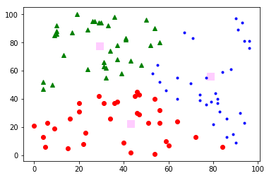
-
Talk61_1.py
Talk61_2.py
Talk61_3.py
- 變數的使用及計算
- 字串使用*號表示複製次數
- True(1)與False(0)首字母需大寫
Recap
第六十二話、decorator
又再來談一下函數,首先看一下以下的例子:def dec1(): for i in range(3): print("這是前面要重複的部分") for i in range(3): print("這是其他部分") for i in range(3): print("這是後面要重複的部分")這是一個函數,其中分為三個部分,第一跟第三個部分是要重複的內容,而中間的是可以變動的內容。討論這個的目的是如果我們有很多的函數都需要使用到重複的部分,那我們是否可以將其另外取出來做成另一個函數,變成函數中的函數。所以我們可以把此函數改寫如下:
def dec2(): for i in range(3): print("這是其他部分") def dec2_repeat(): for i in range(3): print("這是前面要重複的部分") dec2() for i in range(3): print("這是後面要重複的部分")此時呼叫dec2_repeat()會得到跟上面函數一樣的結果。不過這樣變成好像重複的部分變成主體,我們把每次要應用到重複部分的函數傳入。所以再改成這樣:
def dec3(): for i in range(3): print("這是其他部分") def dec3_decorator(func): def dec3_repeat(): for i in range(3): print("這是前面要重複的部分") k = func() for i in range(3): print("這是後面要重複的部分") return k return dec3_repeat dec3 = dec3_decorator(dec3)dec3是非重複部分,每次我們將此部分傳入重複部分並傳回一個新的dec3,此新的dec3包含了原內容與需要重複的部分。現在執行dec3()會得到一樣的內容。在Python中提供我們簡化的寫法,稱為decorator。寫法如下:
@dec3_decorator def dec4(): print("這是dec4的專有內容")執行:
dec4()唔,這太方便了,只要在函數前面加上@decorator,就可以達到跟之前一樣的效果,而且可以不斷地使用,例如再宣告一個函數:
@dec3_decorator def dec5(): print("這裡是dec5的內容")可以重複地使用decorator來將不同程式包覆。當然如果我們不這樣做,難道就不能建立函數?以前的做法用得好好的,反正只是多做幾次copy&paste罷了,何必再多學這個來擾亂自己?Well,搞熟了這個寫法,程式看起來自然簡潔了許多,對於程式的內容編排與理解也會有幫助,所以還是值得了解。
既然如此,再看一下如果函數需要輸入參數的情況:
def dec6_decorator(func): def dec6_repeat(content): print("這��前面要重複的部分") func(content) print("這��後面要重複的部分") return dec6_repeat @dec6_decorator def dec6(content): print(content)之前的重複部分為了要看起來內容比較多,所以用for loop讓它印三次,現在簡化只印一次。執行dec6():
dec6("DoReMi")不過這個寫法有點問題,因為我們必須傳入一個參數到dec6_repeat(),那如果我們使用了另一個函數如下:
@dec6_decorator def dec6_1(content1, content2): print(f"{content1}, {content2}")這個函數需要輸入兩個參數,此時若是執行此函數,將會出現錯誤。難道我們要到dec6_repeat()把輸入參數變成2個?但若是下一次有一個需要輸入三個參數地的函數……還好我們學過不定長度參數的函數設計方式,只要把dec6_repeat()內的參數改為不定長度就好了,修改後如下:
def dec6_decorator(func): def dec6_repeat(*arg): print("這是前面要重複的部分") func(*arg) print("這是後面要重複的部分") return dec6_repeat啊哈,現在我們無論輸入幾個參數都可以了。其實如果我們考慮還有未定長度關鍵字參數,用以下寫法更完整:
def dec6_decorator(func): def dec6_repeat(*arg, **kwarg): print("這是前面要重複的部分") func(*arg, **kwarg) print("這是後面要重複的部分") return dec6_repeat(*arg,**kwarg)這兩個的組合根本就是撲克牌裡面的鬼牌了,可以包括所有的輸入類型。而decorator除了用在函數,也可用於方法(也就是類別內的函數),例如:
class AClass(): @dec6_decorator def aMethod(self, c1, c2, c3): print(f"{c1},{c2},{c3}")簡單測試看看:
ac = AClass() ac.aMethod('Do','Re','Mi')現在舉個現實一點的例子,例如之前我們提到執行程式總會需要計算執行時間,我們可以設計一個計算時間的decorator如下:
import datetime def RunningTime(func): """ Decorator -- For Talk 62 """ def cputime(*arg, **kwarg): start = datetime.datetime.now() func(*arg, **kwarg) stop = datetime.datetime.now() print(f"Running Time = {stop-start}") return cputime嗯,現在可以來試試看,使用以下的程式碼:
@RunningTime def dec7(iteration = 1000000): test = [] for i in range(iteration): test.append(i) for i in range(iteration): test.pop() return test也試著將此decorator加入到之前一話的Talk61_3.py中,並應用到kMeans中的process()方法,請自行參照。
-
Talk62_1.py
- 設計decorator函數來包覆其他函數,只要在函數的上方加上@decorator即可應用decorator內之內容
Recap
第六十三話、喋喋不休的decorator
上一話介紹了decorator的用法,先再舉一個例子:def logged(func): def with_logging(*args, **kwargs): print(f"呼叫函數{func.__name__}") return func(*args, **kwargs) return with_logging這是個拾人牙慧的例子,這個decorator會在某函數執行時顯示函數被呼叫的字樣,例如:
@logged def greeting(name): print(f"Hello, {name}")執行程式:
greeting("Tom")這部分在上一話我們就學會了(`・ω・´),這裡要提的是如何同時使用超過一個decorator的方法。要疊加超過一個decorator,其實只要多寫一行就好了,借用上一話的RunningTime()以及dec7()可以寫成這樣:
@logged @RunningTime def dec7(iteration = 1000000): test = [] for i in range(iteration): test.append(i) for i in range(iteration): test.pop() return test執行dec7():
dec7()唔,有點怪,不是呼叫dec7(),怎麼顯示了cputime?原來使用decorator會覆蓋原來函數的部分訊息,例如__name__,此外,兩個decorator還有執行順序之分,上例應該是這樣logged(RunningTime(dec7)),也就是RunningTime(dec7)是logged的參數,或說是自內向外逐個執行。所以在使用logged()時,RunningTime(dec7)的函數是cputime。要正確顯示可以直接將兩個decorator順序調換即可,反正在這裡誰先誰後沒甚麼差。像這樣:
@RunningTime @logged或者是使用functools模組中的wraps這個decorator,它可以直接讓我們保留元函數名不被換掉,做法是加上這一行:
import functools as ft然後在cputime()方法前加上這個decorator即可:
@ft.wraps(func) def cputime(*arg, **kwarg):現在再執行就沒有錯誤了。
之前提到的decorator都是函數,其實也可以是class。舉例如下:
class Decorator(object): def __init__(self, func): self.func = func def __call__(self): print('這是前面要重複的部分') self.func() print('這是後面要重複的部分')要記得必須使用__call__()方法才行。接著設計要被裝飾的函數:
@Decorator def dec8(): print('Whatever')現在執行dec8()即可得到我們要的結果。與之前類似,可以想見這個decorator的效果與dec8 = Decorator(dec8)的效果是相同的。
-
Talk63_1.py
- 一個函數可以被超過一個的decorator裝飾,執行順序由內往外
- Decorator也可以是class,但必須實現__call__()方法
Recap
第六十四話、永不嫌晚的老生常談
又到了老生常談時間,這次來玩個輕鬆點的遊戲(Talk64_1.py)。有個撲克牌遊戲稱為梭哈,我們的任務是寫一個程式設計一副撲克牌,每一次發牌需隨機選出5張,然後判斷此為何牌型。聽起來不難,因為是撲克遊戲,一副牌有52張牌,顯然我們需要一個撲克牌的class,設計如下:class Card(object): """ 一張撲克牌的物件 """ def __init__(self, suit, rank): self.suit = suit self.rank = rank def __repr__(self): return f"{self.suit}{self.rank}" __str__=__repr__有了一張牌的class,就能建立一副牌的物件,一副牌有52張,也就是需要一個list安裝一整副牌。在這之前,先找到四個花色的unicode代碼,並將花色也儲存在一個list內,如下:
spade = "\u2660" heart = "\u2665" diamond = "\u2666" club = "\u2663" suits = [spade, heart, diamond, club]接下來建立一副牌:
cards = [] for s in suits: for r in range(1,14): cards.append(Card(s, r))現在執行後查看cards就會看到一整副牌了。再來就是隨機取5張牌了,想到隨機自然想到要import random,然後可以使用random.random()來產生隨機數,只要將此隨機數乘以52再取整數的部分,這樣不就是隨機了?
import random as rd cards[int(rd.random()*52)]聽起來蠻好的,不過在list內隨機取一個的函數本來random中就有了,那就是random.choice()。測試一下:
rd.choice(cards)雖然這樣彷彿是可行的,可惜最後可能會出錯。甚麼錯呢?因為要選擇5張,有可能選到同一張牌。那還是每張都確認看看是否已經選過了?像這樣:
def pick(): pick5 = [] index = 0 while True: picked = rd.choice(cards) if (picked not in pick5): pick5.append(picked) index += 1 else: continue if index == 5: return pick5 k = pick() print(k)其實這樣是可行的,因為52取5,重複取到的機率並不算高,要湊成5張不同的牌並不難,只是有可能會多做幾次。因此這裡採用以下方式,雖然在此不見得比上個方法快,但是比較穩妥,做法如下。首先先在Card物件內加上一個新的參數,然後在class中加上比較大小的函數,如在第四十九話中所述。這是要做甚麼?想法是賦予參數一個隨機值,然後根據這個隨機值來排序所有撲克牌,排完之後整副撲克牌便會隨機排列,此稱為洗牌(shuffle)。然後取前5張牌就可以了,因為需要洗牌,所以需要設計比較兩張牌大小的函數,讓兩張牌可以比較大小。因此,class Card修改如下:
class Card(object): """ 一張撲克牌的物件 """ def __init__(self, suit, rank): self.suit = suit self.rank = rank self.ran = None def __repr__(self): return f"{self.suit}{self.rank}" def __lt__(self, anotherCard): if self.ran < anotherCard.ran: return True else: return False def __gt__(self, anotherCard): if self.ran > anotherCard.ran: return True else: return False __str__=__repr__比較大小有大於、小於、大於等於、小於等於等方法,測試了一下,只要寫一個方法就可以用來排序,這裡示範寫兩個,你可以自己測試。接下來就可以直接將cards這個list排序,做法如下:
for c in cards: c.ran = rd.random() cards.sort(key = lambda x: x.ran)有了洗過牌的一副牌,前5張就是我們要的。不過跟大家報告一個好消息,原來洗牌的方法我們在第五十三話中有學過,也就是其實只要我們呼叫rd.shuffle(cards)就可以將其洗牌了,也就是剛剛都是白做的。不過多練習總是好的,現在我們使用以下方式得到5張牌,準備來判定牌型。
rd.shuffle(cards) pick5 = cards[:5]看一下pick5的內容:
pick5嗯哼,這正是我們需要的。到底5張牌可以有哪些牌型?原則上可分為Loyal Flush、Straight Flush、4 of a kind、Full House、Flush、Straight、3 of a kind、Two pairs、One pairs (Jacks or Better)、Nothing。我們一個一個討論。
首先最簡單的大概就是Flush(同花)了,只要5張牌的花色都相同就算。做法是:
if pick5[0].suit==pick5[1].suit==pick5[2].suit==pick5[3].suit==pick5[4].suit: print("It is a Flush") else: print("Not a Flush")暫時先回傳訊息,之後整理時再視程式結構調整。此外,之前提過在Python中提過要比較多個物件是否相等,可以如上這樣一路等於下去,不需要使用and,相當便利。
學會了同花,再來討論Straight。順牌的例子好比說2,3,4,5,6,就是後一張牌的rank剛好是前面一張牌的rank+1,所以只要我們將拿到的5張牌依據點數大小排序,然後看看是否後一張是前一張+1即可。要注意的一點是在梭哈遊戲中,AKQJ10這5張牌是最大的順牌,如果排序後會出現A10JQK,此狀況需另外考慮。了解了之後,做法如下:
pick5.sort(key=lambda x: x.rank) if all([pick5[0].rank==1, pick5[1].rank==10, pick5[2].rank==11, pick5[3].rank==12, pick5[4].rank==13]): print("It is a Straight") elif pick5[0].rank+4==pick5[1].rank+3==pick5[2].rank+2==pick5[3].rank+1==pick5[4].rank: print("It is a Straight") else: print("It is not a Straight")這一段稍長一點,不過應該很容易理解,第一個if測試是否A10JQK,使用all()函數寫起來比較短,也可以用and。第二個if也是為了讓程式碼短一些,當然也可以使用pick5[0].rank+1==pick5[1].rank and …這樣的語法。
接下來就簡單許多了,首先來看Royal Flush(同花大順),原則上這就是同花加上A10JQK的組合,只要我們能夠判斷這兩個就可以判斷是否為Royal Flush。而Straight Flush(同花順)更是順跟同花的組合。
其他的牌型就都不牽扯花色,譬如4 of a kind(閩南話稱為鐵支)在5張牌依據點數大小排序之後,便可以容易地看出。判斷方法就是看前面4張或是後面4張是否點數相同,做法如下:
if (pick5[0].rank==pick5[1].rank==pick5[2].rank==pick5[3].rank or pick5[1].rank==pick5[2].rank==pick5[3].rank==pick5[4].rank): print("It is a 4 of a kind") else: print("It is not a 4 of a kind")按照類似的邏輯,3 of a kind也可以輕易的判斷,若是牌型是3 of a kind,三張同點數的牌在排序之後一定會落在前三張、後三張、或是中間三張。Full House的判斷法也是相同,只有兩種情況,前兩張相同且後三張相同或是前三張相同且後兩張相同,語法如下:
if ((pick5[0].rank==pick5[1].rank and pick5[2].rank==pick5[3].rank==pick5[4].rank) or (pick5[0].rank==pick5[1].rank==pick5[2].rank and pick5[3].rank==pick5[4].rank)): print("It is a Full House") else: print("It is not a Full House")Two Pairs的情況也差不多,需要判斷122、212、221三種狀況(相信你能意會我的意思),如下:
if ((pick5[0].rank!=pick5[1].rank==pick5[2].rank!=pick5[3].rank==pick5[4].rank) or (pick5[0].rank==pick5[1].rank!=pick5[2].rank!=pick5[3].rank==pick5[4].rank) or (pick5[0].rank==pick5[1].rank!=pick5[2].rank==pick5[3].rank==pick5[4].rank)): print("It is a Two Pair.") else: print("It is not a Two Pair")通常這樣的電腦遊戲有得分的One Pair必須是大於Jack的,所以稱為Jacks or better。因此不能只判定是不是有一對,還要再判斷是怎樣的對,所以做法如下:
if (((pick5[0].rank==pick5[1].rank!=pick5[2].rank!=pick5[3].rank!=pick5[4].rank) and (pick5[0].rank==1 or pick5[0].rank >10)) or ((pick5[0].rank!=pick5[1].rank==pick5[2].rank!=pick5[3].rank!=pick5[4].rank) and (pick5[1].rank==1 or pick5[1].rank >10)) or ((pick5[0].rank!=pick5[1].rank!=pick5[2].rank==pick5[3].rank!=pick5[4].rank) and (pick5[2].rank==1 or pick5[2].rank >10)) or ((pick5[0].rank!=pick5[1].rank!=pick5[2].rank!=pick5[3].rank==pick5[4].rank) and (pick5[3].rank==1 or pick5[3].rank >10))): print("It is Jacks or Better") else: print("It is not Jacks or Better")至於完全不符合上述任何一種的牌型就是Nothing了。接下來跟之前一樣,在Talk64_2.py中重新整理讓其成為一個完整的程式。原則上還是整理成為兩個class,巧合,完全是巧合。第一個當然是Card,為了讓顯示更為逼真,把其中的__repr__()做了點修改,如下:
def __repr__(self): if self.rank == 11: return f"{self.suit}J" elif self.rank == 12: return f"{self.suit}Q" elif self.rank == 13: return f"{self.suit}K" elif self.rank == 1: return f"{self.suit}A" else: return f"{self.suit}{self.rank}"第二個class名為ShowHand,其初始狀態如下:
class ShowHand(object): def __init__(self): self.cards = []#建立一副牌 self.pick5 = []#取出5張牌 for s in suits: for r in range(1,14): self.cards.append(Card(s, r))在此class中,建立一個private方法來洗牌並取得隨機5張牌:
def __shuffle(self): """ 洗牌 """ rd.shuffle(self.cards) self.pick5 = self.cards[:5]此外也建立另一個private方法來將pick5中的牌按照點數排序:
def __sortByRank(self): """ Sort pick5 by Rank """ for p in self.pick5: p.ran = rd.random() self.pick5.sort(key=lambda x: x.rank)在class中加入所有判斷不同牌型的方法,在此全都設為private,因為這些方法都只會在這個class內被呼叫。除了__isStraight()這個方法之外,其他的判斷牌型方法的傳回值都是True or False。而__isStraight()則傳回1(大順)、2(一般順)、0(非順)。這些都有了之後,建立一個方法來總理判斷牌型如下:
def __judge(self): """ 判斷牌型 """ self.__sortByRank() if self.__isRoyalFlush(): return "同花大順" elif self.__isStraightFlush(): return("同花順") elif self.__is4OfAKind(): return("鐵支") elif self.__isFlush(): return("同花") elif self.__isStraight(): return("順") elif self.__is3OfAKind(): return("三條") elif self.__isTwoPairs(): return("Two Pairs") elif self.__isJacksOrBetter(): return("Jacks or Better") else: return("Nothing")這個方法會傳回牌型。最後加上一個public的方法讓外部呼叫:
def deal(self): """ 發牌 """ self.__shuffle() j = self.__judge() print(f"{j}\n{self.pick5}") return j這個方法會印出牌型與所得到的5張牌,順便傳回牌型。為了讓使用者更有感覺,設計一個簡單的介面,可以輸入發牌或是結束。
if __name__=="__main__": #""" sh = ShowHand() while True: command = input("Deal(d) or Quit(q)?") if command.casefold() == "Deal".casefold() or command.casefold() == "d".casefold(): sh.deal() if command.casefold() == "Quit".casefold() or command.casefold() == "q".casefold(): break #"""現在可以執行程式了。若要延伸這個遊戲,有一種玩法是可以讓玩家蓋掉幾張牌然後重發,請自行思考設計。此外,為了確認每一種牌型都可以判斷出來,在主程式使用以下的程式碼,記得要先comment掉剛剛介面的部分:
#""" @RunningTime def check(): sh = ShowHand() while True: if sh.deal().casefold() == "同花大順".casefold(): break check() #"""請自行修改要確認的牌型,例如輸入同花。這個函數有加了個decorator(@RunningTime),就是上一話寫過的,你應該印象深刻。這個函數會一值執行直到找到想要確認的牌型為止。同花大順真的是靠運氣,有一次試了好幾分鐘才找到, 或許可以再增加計算要發幾次牌才會得到某牌型,多跑幾次看看機率跟以前學的機率是不是很接近。
第六十五話、Regular Expression - 1
之前提過分割字串的方法,再來回味一下。s = "One little Two little Three little Indians" s.split("little")不過如果不小心打錯字變這樣:
s = "One Little Two litttle Three litle Indians"好像還有點規律,不過split()便不敷使用了。意思是如果找到一點規律,還是可以分拆。而Regular Expression便提供此用途。有非常多的程式語言支援regular expression的使用,而Python中的regular expression內容收集在re這個模組,所以只要將此模組import進來即可使用。Re的功能很強大,可以更簡便的協助處理字串,若是觀察其help(re),可以看到許多內容跟符號介紹,原則上多使用就會記得,反正記不得再查就好了。接下來還是先從看一個例子入手:
import re s = "One Little Two litttle Three litle Indians" lista = re.split(r'lit+le',s) print(lista)Re中也有一個方法叫做split(再次說明有Name space的好處,雖然re.split跟s.split我們還是不會搞錯),此方法的說明:
help(re.split)如果懶得讀這些英文,意思就是輸入一個pattern當作第一個參數,輸入一個字串當作第二個參數,然後找到符合pattern的子字串來當作delimiter來分拆這個字串。我們使用的pattern寫法就是r’lit+le’,前面的r表示這個字串是raw string,在Python中通常就是用這種raw string來表示pattern。接著再看裡面的lit+le,這裡面的+號表示前一個字元出現一次或超過一次。也就是t出現一次或多次的情形。因此,litle、little、little、甚至littttttle都包含在此pattern內。聽起來符合我們的需求,看一下結果:
['One Little Two ', ' Three ', ' Indians']
唔,不太對,Little的L是大寫,看來是不在上述pattern能夠偵測的範圍。解決的辦法是要讓其忽略大小寫,如下:
lista = re.split('lit+le',s, flags = re.IGNORECASE)現在再看結果就沒錯了。從這裡延伸一下,剛才提到+號是至少一個,但若是*號的話就是至少0個。所以如果使用r’lit*le’的話,會包含lile(t出現0次)。好比說:
s = "One Little Two litttle Three lile Indians" lista = re.split(r'lit*le', s, flags = re.IGNORECASE) print(lista)再看一個變化:
s = "One Little Two litttle Three litle Indians" lista = re.split(r'(lit+le)',s, flags = re.IGNORECASE) print(lista)Pattern加上小括號?結果如下:
['One ', 'Little', ' Two ', 'litttle', ' Three ', 'litle', ' Indians']
OK,原來這樣做的話會保留pattern在傳回的list內。其實這個結果不就是根據空白來分割嗎?要根據空白分割,即使空白包含space+tab,這個時候其實使用s.split()最簡單,這裡還是試一下re的做法:
s = "One\t Little \t Two litttle \t Three litle \t Indians" lista = re.split(r'\s+',s) print(lista)這裡的\s是表示空白(space)的意思,在Python中有幾個這樣的特定字元(使用\來表示),以下為常用的幾種:
| 符號 | 意義 | 等同 |
| \d | 表示數字 | [0-9] |
| \D | 表示非數字 | [^0-9] |
| \w | 表示數字、字母、底線 | [a-zA-Z0-9_] |
| \W | 表示非\w | [^a-zA-Z0-9_] |
| \s | 表示空白 | [\r\t\n\f] |
| \S | 表示非空白 | [^\r\t\n\f] |
lista = re.split(r'\W+',s)來得到一樣結果,\W表示不是數字字母,在這個字串中就只剩下空白了。接著來試試看數字:
s = "1 Little 2 litttle 3 litle Indians" lista = re.split(r'\d',s) print(lista)顯示結果如下:
['', ' Little ', ' litttle ', ' litle Indians']
雖然1前面沒東西,不過還是會被分割出一個空字串,此外其中的空白也依然存在,可以這樣修改:
lista = re.split(r'\s*\d\s+',s)空白沒了,不過第一個空白字串還是存在。那若是使用\D呢?
lista = re.split(r'\D+',s) # ['1', '2', '3', '']這看起來就容易多了,把文字去掉,數字抓出來。容易,不過剛剛的表格中後面有個等同,其中的中括號又是甚麼意思?中括號的意思是比對,也就是說比對出跟中括號內所要表示的字串相同的字串,而在中括號內加上^,則表示比對出跟中括號內所要表示的字串不同的字串。所以[0-9]就是表示所有數字[a-z]表示所有的小寫英文字,若是寫[a-zA-Z0-9_]則表示所有數字字母底線。來看看怎麼應用:
s = "1 Little 2 litttle 3 litle Indians" lista = re.split('\s*[0-9]+\s+',s) # ['', 'Little', 'litttle', 'litle Indians'] print(lista)這個效果跟r'\s*\d\s+'相同,也就是內容是純粹數字的子字串都是用來分割字串的delimiter。忘了加上r來定義其為raw string,不過一樣可以使用,看來頗有彈性ヽ(^。^)ノ。若是使用否定句,則效果如下:
lista = re.split('\s*[^0-9]+\s*',s) # ['1', '2', '3', '']
-
Talk65_1.py
- Import re來使用regular expression
- re.split(pattern, string)也可用來分割字串
- 使用+、*、\s、\S、\d、\D、\w、\W、[]、[^]等符號組合來建立pattern
Recap
第六十六話、Regular Expression - 2
Re常用來尋找某類型字串,譬如在一篇文章中,我們想要知道其中有哪些電話或是某些人名出現次數等等,所以接著我們來看搜尋的函數。第一個出場的是findall()函數,解釋如下:help(re.findall)顧名思義就是要找到全部符合pattern描述的子字串,並將其傳回至一個list內。例如假設我們有以下字串:
s = '''台灣大學 10617台北市大安區羅斯福路四段1號TEL:02-3366-3366 清華大學 30071新竹市東區光復路二段101號TEL:03-571-5131 交通大學 30071新竹市大學路1001號TEL:03-571-2121 成功大學 70101台南市東區大學路1號TEL:06-275-7575 '''現在我們想要知道裡面有哪幾間大學?可以試著這樣做:
university = re.findall(r'..大學',s)..是啥?原來.是萬用牌啊,也就是撲克牌裡的鬼牌,所以只要大學前面有兩個東西(無論是數字文字或空白都算)。當然我們可以使用前面的\w應該會比較精確,像這樣:
university = re.findall(r'\w\w大學',s)\w\w表示前面有兩個字(可以想像如果這個大學名字不是兩個字就會只抓到前面兩個字,例如柏克萊大學、早稻田大學之類,不過這裡還算OK),執行看看:
print(university)咦,出現了奇怪的大學?仔細一瞧,原來是地址。這樣的話,再看一次,還好大學名後面有個空白,所以改成這樣:
university = re.findall(r'..大學\s', s)這次好多了,雖然每個大學後面都有一個空白,但是至少都對了,而且我們可以使用strip或rstrip來將空白去除。接著來試著找出郵遞區號,剛好都是5碼,如果沒有其他規則,那5個數字就是共同點:
zipcode = re.findall(r'[\d]{5}', s){5}的意思就是乘以5倍,也就是有5個數字,在此例中[]有無並不影響。接下來再試著找出所有電話,因為電話有格式,所以也不難:
phone = re.findall(r'0\d-\d{3,4}-\d{4}', s)\d{3,4}的意思是3到4個數字,因為台北多一碼,所以這樣才抓得到。當然也可以這樣簡化:
phone = re.findall(r'0\d-\d+-\d+', s)若是要找新竹的電話,則使用
phone = re.findall(r'03-\d+-\d+', s)下一個相關函數是match(),此函數是要找出某字串是否符合某pattern,但自字串開頭開始比對,找到傳回一個match物件,若是沒找到則傳回None。例如:
slist = re.split('\s*\n\s+', s)[:-1] for ele in slist: z = re.match(r"(\w{2}大學)\s([\d]{5}.+)TEL:(0\d-[\d]+-[\d]+)",ele) if z: print(z.groups())第一步是利用re.split()將s的內容分割後放入slist這個list內,內容如下:
print(slist)接下來使用re.match()針對每一個元素進行比對,pattern內的小括號是指將比對符合的部分存入一個變數,最後傳回一個match物件,此物件有一個方法稱為groups(),會傳回其內元素所形成的tuple。
一個tuple中包含三個部分,分別是適才小括號內格式的內容。假設將match內容改為:
z = re.match(r"(\w{2}大學)\s([\d]{5}.+)TEL:(03-[\d]+-[\d]+)",ele)最後一個是search(),這個函數也是找尋match,只是不是字開頭比對,而是走遍整個字串來找是否有match,找到傳回match物件,否則傳回None。例如:
pattern = r'0\d-[\d]{3}-[\d]{4}' match = re.search(pattern, s)執行:
print(match.group())僅傳回第一個符合pattern的子字串,使用match.group()來取得。另一個尋找match的方法是sub(),是代換的意思,也就是找到之後用另一個字串取代它,例如:
pattern = r'TEL:' newInfo = re.sub(pattern, '', s)這意思就是找到符合TEL:的子字串,然後用空字串''來代替它,也就是去除了,現在查看newInfo,可以看見其中的TEL:部分被去除了。另一個函數finditer()會傳回所有符合的字串的iterator,如下:
pattern = r'0\d-[\d]{3}-[\d]{4}' for m in re.finditer(pattern, s): print(f"{m.start()}-{m.end()}, {m.group(0)}") # 0 for the entire matchm.start()與m.end()方法傳回符合的match之起始與結束位置。
Regular Expression還有其他符號與變化,就不再這裡一一詳述,你可以使用help(re)查看其他符號,或是上網搜尋。
-
Talk66_1.py
- re.findall(pattern, string)可以找到字串中所有符合pattern的子字串並傳回list
- re.match(pattern, string)可以判斷字串是否符合pattern並傳回match物件或None
- re.search(pattern, string)可以判斷字串中是否有符合pattern的子字串並傳回match物件或None
- re.sub(pattern, repl, string)可以將字串符合pattern的子字串使用repl代換並傳回新字串
- re.finditer(pattern, string)可以找到字串中所有符合pattern的子字串並傳回iterator
Recap
第六十七話、NamedTuple
之前提過一些容器例如list、tuple、set、dictionary等,其中排成一列並使用有順序的標記之資料型態,稱之為sequence type ( 在Python中包含strings、Unicode strings、lists、tuples、bytearrays、buffers、 and xrange objects),而set與frozenset則稱為set type,dict則稱為mapping type,因為我們用key來對應value。這些容器的主要作用就是用來儲存排列資料,因應不同的使用目的,我們會選擇使用不同的容器。對於資料,我們最常做的三件事情是加入、刪除、與搜尋,例如我們有一本字典,裡面當然收藏很多字,此時對於我們來說,搜尋查詢可能是最重要的一件事情,因為做得最多次,所以我們希望字典的排列非常適合我們搜尋,可以讓搜尋變快,雖然有時候會加新字,但是畢竟機會較少,因此這方面的操作速度沒那麼快也就馬馬虎虎了。
因此,除了之前介紹的幾種資料結構之外,Python還提供了一些其他的資料結構收藏於collections這個模組,而除了這些之外,還有各種其他種類的資料結構,不過Python沒提供的話可能就得自己寫了。這裡僅介紹Python提供的,若想進一步了解可尋找資料結構相關的課程或資料。 Collections這個模組包含了以下幾種資料結構:namedtuple、deque、ChainMap、Counter、OrderedDict、defaultdict、UserDict、UserList、與UserString等。這裡來談談namedtuple,這個名稱聽起來顯然跟tuple有關,所以內容是不可以改變的(immutable),不過這個tuple有甚麼不同?比方說,之前我們做過一些例子關於平面上的點,主要的屬性是x跟y,對於某一點p來說如果使用tuple來表示可以寫成p=(x,y),不過只是兩個數字,無法看出跡象是代表座標,如果要描述的內容再多一些(例如再加上編號、需求等屬性),可能就會搞混了。
各位一定心想:阿不是可以寫一個class就解決了,像這樣:
class Node(object): def __init__(self, x, y): self.x = x self.y = y當然你是對的,不過也可以不需要這樣慎重其事,namedtuple提供我們一個簡便的方法。舉例如下:
from collections import namedtuple as nt # 建立一個namedtuple (類似class) Node = nt('Node', ['x','y']) # 產生一個namedtuple物件 n = Node(x = 1, y = 2) # p = Node(11, 22)首先當然要先import namedtuple,這當然沒問題。接著看一下nametuple的help:
help(nt)第一個參數是typename,我們使用Node,第二個是field_names,使用['x','y'],然後傳回一個新的subclass。也就是說其實我們建立了一個新了class,是一個tuple,但是有包含名稱。跟我們設計一個名為Node的class然後包含x、y兩個參數意思差不多,只是是使用tuple,所以內容無法更改。現在測試一下:
print(n.x) print(type(n)) n.y = 20嗯哼,跟我們想的一樣。現在等於我們有一個Node物件了,我們便可以使用這物件來儲存點資料(但是無法修改)。接下來來看一下它的方法,第一個方法可以讓我們把iterable物件變成namedtuple,例如:
# 使用_make()將iterable物件變成namedtuple物件 xy = [10, 20] n1 = Node._make(xy) print(n1)_make()可以產生一個新的Node。也可以將dict轉為namedtuple物件,例如:
# 將dict變成namedtuple物件 xydict = {'x':100, 'y':200} n2 = Node(**xydict)若是反過來想將namedtuple物件變成dict,則使用_asdict()方法:
# 將namedtuple物件變成dict dic1 = n1._asdict() print(dic1)唔,不是dict,原來在Python3.1版的時候改為傳回OrderedDict,這個之後再提,不過也別擔心,它還是一種dict。
雖說namedtuple內容不可變,不過還是可以使用_replace()方法改變:
# 建立一個新內容的namedtuple物件 print(id(n2)) n2 = n2._replace(x=101) print(id(n2))這裡特別將n2的id印出,可以看出使用_replace()之前與之後的id不相同,所以原則上並不是修改內容,而是讓指標指向另一個物件。若想查看這些方法內容,可以在建立之時讓verbose=True,將會在console顯示相關資料。現在我們試著應用namedtuple到之前第53話的例子(Talk67_2.py),可以初始化其中的點如下:
import random as rd from collections import namedtuple as nt Node = nt('Node', ['id', 'x','y']) class Route(object): def __init__(self, nNodes = 20): self.nNodes = nNodes self.nodes = [] self.initialize() def initialize(self): rd.seed(20) x = [rd.randint(0, 100) for _ in range(self.nNodes)] y = [rd.randint(0, 100) for _ in range(self.nNodes)] for i in range(self.nNodes): self.nodes.append(Node(i, x[i], y[i])) def distance(self, a, b): return ((a.x-b.x)**2+(a.y-b.y)**2)**0.5使用namedtuple讓我們少寫了一個class Node,看起來蠻好的。不過若是應用到第61話的話(Talk67_3.py):
from collections import namedtuple as nt Node = nt('Node', ['id', 'x','y', 'group']) class kMeans(object): def __init__(self): self.nodes = [] self.initialize() def initialize(self): with open("T61_nodes.txt", 'r') as f: for line in f: record = line.split(',') nid = int(record[0]) x = int(record[1]) y = int(record[2]) self.nodes.append(Node(nid, x, y, -1)) def distance(self, a, b): return ((a.x-b.x)**2+(a.y-b.y)**2)**0.5看來似乎都一樣,不過這裡的Node有一個參數group是經常要更換其值的,所以如果要換值的話則:
k.nodes[0] = k.nodes[0]._replace(group=1) print(k.nodes)還是可以,不過看起來麻煩了點,而且會一直需要產生新的物件,所以可能還不如寫一個class了。
-
Talk67_1.py
Talk67_2.py
Talk67_3.py
- 從collections內import namedtuple
- 使用namedtuple(typename, field_names)方式來建立class
- 可以使用_make()來建立物件
- 使用 (**dict)與_asdict()來與dict互相轉換
- 使用_replace()來改變內容,但會產生新物件
- 若是需要經常修改物件內容,自訂class可能較為容易
Recap
第六十八話、deque
Deque是double-ended queue的簡稱,可以用來模擬queue跟stack,這裡先提一下何謂queue跟stack。Queue的意思就是行列,就像我們排隊買電影票一樣,資料就是列隊中的人,而這個行列最主要的操作就是自後加入以及自前移除,就像有人加入排隊買票以及前面買好票就離開隊伍一樣。這是所謂的先來先服務或說先進先出(First in, first out(FIFO)),就像水管裡的水一樣。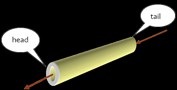
Stack跟queue類似,也是一個行伍,而不同的地方就是stack是先進後出(First in, last out(FILO)),如圖:
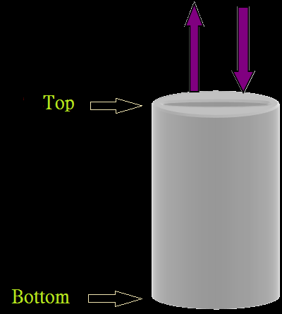
stack與queue的另一個不同處是stack總是只操作一端,就像坐電梯,先進去的後出來,且只有一個門可以進出。了解了這個概念之後,我們就納悶了,這不是都可以使用list來實現嗎?當然是可以,不過list在操作插入與刪除元素速度較慢,而deque可高效實現插入與刪除操作。至於做法就不難了,舉例如下:
from collections import deque q = deque(list(range(3))) q.append(5) q.appendleft(100)首先一樣的起手式,先import才能使用。再看一下deque的help:
help(deque)宣告的時候可以給一個iterable物件,若是沒給表示初始是一個空的deque。跟list一樣使用append,會將新的元素加到後面,若是使用appendleft(),則將新元素加到左邊(前面),當然也可以使用insert(0, 100)來代替。若是一開始設定了maxlen屬性,會怎麼反應?
q1 =deque(list(range(6)), maxlen = 5)看一下目前情況:
print(q1)裡面沒有0,表示第一個參數iterable內的元素是一個一個append到deque內,因為有最長長度限制,所以append後就從前面擠掉一個了。再如:
q1.append(6) print(q1) q1.appendleft(-1) print(q1)再append一個,又從前面擠掉一個,但若是appendleft,就從後面擠掉一個,長度則一直保持是5。接下來是移除,我們可以使用pop()與popleft(),例如:
print(q1.pop()) print(q1.popleft())Pop()會傳回被移除的物件,此時檢查q1則:
print(q1)現在可以歸納如果是queue要加入元素(稱為enQueue)則使用append(),若是要移除元素(稱為deQueue)則使用popleft()。若是stack則要加入元素(稱為Push)則使用appendleft(),若是要移除元素(稱為Pop)則使用popleft()。當然你想要反方向也可以,例如stack加入使用append(),移除使用pop()。
Deque包含數個與list相同的方法,例如clear、copy、count、index、remove、reverse等,也有些有相異處的,例如insert()。之前提到也可以用insert(0, x)來將x加入到最前面,不過當我們有設定maxlen且目前已經到達maxlen則無法使用insert(0,x)來加入,但是可以使用appendleft()。例如:
q1.insert(0, 200)此外,可以使用extend()以及extendleft()來加入元素。例如:
q1.extend([7,8,9]) print(q1) q1.extendleft(['a','b','c']) print(q1)除了可以看出extend系列都是逐一加入新iterable內的元素,且可以使用extendleft()來變成自前方加入。最後再說一個list沒有的方法稱為rotate(),此方法是將內容元素平移數個,若是負的則往右移動,例如:
print(q1) q1.rotate(2) print(q1) q1.rotate(-2) print(q1)應該很容易可以看出差別。
-
Talk68_1.py
- 使用deque來模擬queue與stack
- 使用append()與appendleft()來增加元素,再使用pop()與popleft()來移除元素
- 可以使用clear、copy、count、index、remove、reverse、insert、extend、extendleft、以及rotate等方法來操作這個queue
Recap
第六十九話、ChainMap
ChainMap是可將數個mappings(例如dict)結合來形成一個單一的view。這些mappings會儲存在一個list內。舉例如下:from collections import ChainMap dict1 = {'one':1, 'two':2} dict2 = {'one':'a', 'two':'b', 'three':'c'} chain = ChainMap(dict1, dict2)一樣先import ChainMap,然後在ChainMap()內加入dict。現在看一下chain的內容:
print(chain) print(chain.maps)maps這個變數儲存ChainMap的內容。因為在設計的時候,給兩個dict重複的keys但是不同的values,所以現在檢查一下:
print(list(chain.keys())) print(list(chain.values()))嗯,重複的key僅出現一次,而其內容則以第一個為準。也就是說排在後面的mapping內容如果跟前面有一樣的key,則以前面的為準。接下來也可以像dict一樣取得內容:
print(chain['two']) print(chain.get('two'))這兩個方式都能得到其中的值。如果我們輸入以下指令呢?
chain['two'] = 'b'再看一下:
print(chain.maps) print(chain.get('two'))嗯,看來也就是僅能動到第一個的值。接下來若是想要再加入一個mapping(dict)呢?可以使用new_child()方法:
dict3 = {'one':1, 'two':2, 'three':3} chain = chain.new_child(dict3)此時再查看一下:
print(chain.maps) print(list(chain.values()))如果想要traverse這個ChainMap,可以如下:
for k, v in zip(chain.keys(), chain.values()): print(k, '->', v) for i in chain: print(i)使用ChainMap來組合dict比使用update()方法來更新速度來得快。
-
Talk69_1.py
- ChainMap可用來組合多個mapping(dict)物件
- 使用maps來觀察組合,使用keys()與values()方法來得到key跟value
- 使用new_child()方法來加入新的mapping
Recap
第七十話、Counter
Counter是dict的subclass,用來計數hashable objects。所謂hashable objects就是在其生命週期內擁有不變的hash value的物品,原則上就是擁有__hash__()方法的物件,簡單的說不會變的是hashable(e.g. int, float, bool, string, tuple, range, frozenset, bytes),而會變的就不是hashable(e.g. list、dict、set)。例如:print('a'.__hash__()) print([1,2,3].__hash__())而Counter就是接收物件當作key,把其計數當作是value。看個例子便了解:
c1 = Counter() print(c1) c2 = Counter('One little, two little, three little indians') print(c2) c3 = Counter(['abc', 'cba', 'aaa', 'abc', 'cba', 'bac']) print(c3) c4 = Counter([[1,2,3], [3,2,1], [1,2,3], [2,1,3], [3,2,1]]) print(c4)c4會出現錯誤因為裡面的元素不是hashable物件,所以無法計數。因為Counter是dict的subclass,所以可以使用dict的方式來查詢:
print(c3['abc']) print(c3['acb'])可以使用elements()方法來得到所有的元素,不過傳回的是一個chain物件,原則上就是個iterator:
print(c3.elements()) print(list(c3.elements())) print(sorted(c3.elements())) for i in c3.elements(): print(i)計數之後便會想到哪一種多,需要簡單統計,此時使用most_common(n)來顯示:
print(c2.most_common(3))參數n如果沒提供的話則會顯示全部。現在看一下應用,我們有一個檔案(file2.txt)其內容如下:
The itsy bitsy spider
Went up the water spout
Down came the rain and
Washed the spider out
Out came the sun
And dried up all the rain
Now the itsy bitsy spider
Went up the spout again
from collections import Counter import re words = re.findall(r'\w+', open('file2.txt').read().lower()) count = Counter(words).most_common(10) print(count)統計結果如下:
[('the', 8), ('spider', 3), ('up', 3), ('itsy', 2), ('bitsy', 2), ('went', 2), ('spout', 2), ('came', 2), ('rain', 2), ('and', 2)]
可以找本小說來試試看。
-
Talk70_1.py
file2.txt
- Counter是dict的subclass,可使用elements()來取得所有元素
- 使用most_common(n)方法來取得出現次數最多的前n名
Recap
第七十一話、OrderedDict
OrderedDict也是dict的subclass,應該從名字就可以猜出來。通常我們建立一個dict後查閱其內容會發現它沒有固定順序,而若是想要有特定順序排序,可以使用OrderedDict。做個例子比較看看:from collections import OrderedDict dic1 = {'one':1, 'two':2, 'three':3, 'four':4} od1 = OrderedDict({'one':1, 'two':2, 'three':3, 'four':4}) print(f"dic1 = {dic1}\nod1 = {od1}")結果看起來一樣(@_@)。再在console查閱一次:
print(dic1) print(od1)如果我們想要排序他們,可以使用sorted()函數:
print(sorted(dic1.items(), key = lambda x: x[1])) print(sorted(dic1.items(), key = lambda x: x[0])) print(sorted(od1.items(), key = lambda x: x[0]))還記得我們可以使用del()、pop()、與popitem()來刪除dict內的元素嗎?現在來刪除一個元素然後再加回去看看:
print(dic1.popitem()) print(od1.popitem())因為最後一個元素不一樣,所以傳回的不同,再把它們加回去之後,看一下狀況:
dic1['one'] = 1 od1['four'] = 4 print(dic1) print(od1)好像都回到原位置了,這次試試看刪除同一個元素:
print(dic1.pop('one')) print(od1.pop('one'))接下來再把元素補回去看看:
dic1['one'] = 1 od1['one'] = 1 print(dic1) print(od1)dic1還是沒變,不過od1中的元素變成最後一個,也就是說變成新元素加到最後了。如果想要把one再移到最前端要怎麼做?在OrderedDict中提供一個方法move_to_end()來將元素移動到兩端,例如:
od1.move_to_end('one', last = False) print(od1)因為last的值是False,所以移到最前端,它的預設值是True,是移到最後端。因為OrderedDict是有序的,所以支援reversed()函數,此函數傳回一個iterator,如下:
for k, v in reversed(od1.items()): print(k, v)當我們更新一個dict內的元素,其實是呼叫了__setitem__()這個方法,在dict中,更新了就更新了,因為沒有特定順序,但是在OrderedDict中,我們希望某元素被更新後變成最後一個,表示它是最近被修改過的,那要怎麼做?其實也不難,就是把舊元素刪除了加上新元素即可,現在來試試看:
class LastUpdatedOD(OrderedDict): def __setitem__(self, key, value): if key in self: #del self[key] self.pop(key) OrderedDict.__setitem__(self, key, value)建立一個繼承自OrderedDict的class,這樣可以保有所有OrderedDict的屬性,只要重載__setitem__()方法即可。現在測試一下:
luod = LastUpdatedOD() luod['one'] = 1 luod['two'] = 2 print(luod) luod['one'] = 10 print(luod)這樣的方式可以讓我們一直追蹤哪個元件是最近被更新的。我們也可以設計一個固定長度的OrderedDict,而且是先進先出(FIFO)的順序,如下:
class FixedLengthOrderedDict(OrderedDict): def __init__(self, capacity): self._capacity = capacity def __setitem__(self, key, value): if len(self) >= self._capacity: last = self.popitem(last=False) print(f"{last[0]}:{last[1]} is removed.") print(f"{key}:{value} is added.") OrderedDict.__setitem__(self, key, value)測試一下:
flod = FixedLengthOrderedDict(2) flod['one']=1 flod['two']=2 flod['three']=3這不就是一個固定長度的Queue嗎?你能夠使用deque來製作類似的結構嗎?此外,也可以將上面兩個class合併,變成一個固定長度且會將最後更新的元素排在最後的Dict。此部分留給各位探索。
-
Talk71_1.py
- OrderedDict可以使用sorted()來排序,使用del()、pop()、與popitem()來刪除元素,使用move_to_end()來將元素移動到兩端
- 藉由設計__setitem__()方法可以設計不同型態的dict
Recap
第七十二話、defaultdict
又是跟dict有關,先來看個例子:mathGrades = {"小杉":100, "胖虎":60, "小夫":80, "靜香":90} students = ["小杉", "胖虎", "小夫", "大雄", "靜香"] for s in students: print(f"{s}的數學成績是{mathGrades[s]}")這個程式片段執行後會出現錯誤,因為大雄缺考,所以沒有登錄到成績。可是只是要看個全班成績或是算個平均,還跳個錯誤出來中斷程式,能否就跳過去就算了?這時考慮使用get(),如下:
for s in students: print(f"{s}的數學成績是{mathGrades.get(s, -1)}")get()有第二個關鍵字參數,預設值是None,所以如果這個key不存在,傳回一個特定值,這裡選擇-1表示成績未定。顯示結果如下:
小杉的數學成績是100
胖虎的數學成績是60
小夫的數學成績是80
大雄的數學成績是-1
靜香的數學成績是90
print(mathGrades)我們希望如果找不到該學生,就直接幫他建立這個key,省得之後還要找哪個缺考再補上去,那要怎麼做?我們可以寫一個函數如下:
def getGrade(key, defaultvalue): if key not in mathGrades: mathGrades[key] = defaultvalue return -1 else: return mathGrades[key] for s in students: print(f"{s}的數學成績是{getGrade(s, -1)}")這樣若是缺考的同學成績便會使用-1記錄下來,現在再看mathGrades內容:
print(mathGrades)這樣無論誰缺考,成績登錄還是會被產生。不過這個用法剛好dict已經幫我們設計好了,名為setdefault()。直接用用看:
for s in students: print(f"{s}的數學成績是{mathGrades.setdefault(s, -1)}")原則上setdefault()這個方法跟get()差不多,都是得到的意思,只是這個方法如果在dict內找不到相同的key,便會在dict內建立這個key,且可以讓我們指定預設值,跟上述的函數用法相同。如果我們一開始就預見可能會有存取到不存在的key這樣的情況,那麼便可以直接使用defaultdict,省下剛剛諸多的操作,如下:
from collections import defaultdict defaultMathGrades = defaultdict(int, mathGrades) print(defaultMathGrades)看一下顯示內容:
defaultdict(
print(defaultMathGrades["大雄"]) print(defaultMathGrades)也就是說這個資料結構defaultdict在一開始建立就構思了初始值,又因為它是繼承自dict的class,所以其他使用皆與dict相同。再看一下它的help,
help(defaultdict)第一個參數是factory,甚麼是factory?在程式設計的定義,Factory Method Pattern就是說使用函數來建立物件。所以像int()、type()、或是list()等,雖然看起來像是函數,但實際上都是一種class,使用它們後會產生該class的物件。除了上述三種,我們熟知的long()、float()、complex()、str()、unicode()、tuple()、dict()、bool()、set()、frozenset()、object()、super()、property()、與file()等,都可稱為工廠函數。了解了這點之後,再試一下建立新的defaultdict如下:
grades = [("小杉",100), ("胖虎",60), ("小夫", 70),("靜香", 95),("小杉", 100)] dd = defaultdict(list) for s, rank in grades: dd[s].append(rank)測試一下看看:
print(dd) dd["胖虎"].append(50) print(dd) print(dd["大雄"]) print(dd)
-
Talk72_1.py
- 使用defaultdict可以在找不到相同key時自動針對預設類型產生該key與其對應的值。
Recap
Python亂談
NumPy
第七十三話、numpy之基本介紹
之前已經介紹了許多資料結構,讓我們可以使用許多不同的方式排列並使用資料。接下來談一談額外的資料處理模組,首先是numpy。Numpy的主要結構是array,原則上就是list,但是我們已經有list了,何必再學一個array?那當然是因為它在某些程度上更強大。在學習之前需先安裝這個package,這也是為何我們選擇anaconda的原因,因為此numpy在安裝anaconda時已經一併安裝了,所以我們可以直接使用。現在我們先從個例子看起:
import numpy as np arr = np.array([1,2,3])要使用numpy必須要先import,而array()是其中的一個方法,用來建立一個新的array。看一下說明內容:
np.array?
注意其參數object是array_like,也就是說像array的資料結構都可以,例如list、range、或是tuple等都可以。看一下arr的內容:
print(arr, "\n", type(arr))若是存取資料也可使用跟list相同的操作,例如:
print(arr[0]) arr[2] = 30 print(arr)看不出來跟list有甚麼不同,除了type名稱不同,怎麼看怎麼像list,現在看一下它的資料型態,使用dtype.name:
print(arr.dtype.name)內容都是整數。到目前為止,看不太出來跟list的分別。接著再看一個例子:
arr1 = np.array([1,2,3.14159]) arr2 = np.array([1,2,"3.14159"])接著看它們的dtype:
print(arr1.dtype.name, "\n", arr2.dtype.name)這說明了一件事就是array裡面儲存的元素資料型態是相同的,即使輸入時不同,它也會自動幫我們轉換,但是我們知道list是可以有不同形態資料的。我們可以看一下它們的itemsize來做進一步的驗證:
print(arr.itemsize, "\n", arr1.itemsize, "\n", arr2.itemsize)Itemsize是指每個資料所需要的位元組(byte)數,例如arr是int32,所以32/8=4,每個資料需要4個bytes。在建立array的時候,也允許我們直接指定資料型態,只需要使用dtype關鍵字即可,如下:
arr3 = np.array([1,2,3], dtype = "float")現在再看其內容則如下:
print(arr3) print(arr3.dtype.name)這樣的形態使得array所需要使用的記憶體空間較少,所以如果我們要運算的資料可以使用相同的型態儲存,使用array可以讓我們更有效率。接下來看另外兩個屬性shape與ndim,shape是指資料排列的形狀大小,ndim是dimension,就是維度。例如:
print(arr.shape, "\n", arr.ndim)Shape為(3,)的意思是因為只有一維,資料有三個。若是維度加大就會顯示不同了,例如:
arr4 = np.array([[1,2,3],[4,5,6]])這顯然是二維的,如下:
print(arr4.shape, "\n", arr4.ndim)Shape變成(2,3),原則上就是2個row,3個column。至於array之中的資料數量,則可以使用size參數得到,例如:
print(arr.size, "\n", arr4.size)現在我們已經了解了array的相關型態內容,這裡好奇的嘗試一下,如果我們使用以下指令來建立array結果會如何?
arr5 = np.array([[1,2,3],[4,5]])會跟arr4的內容雷同嗎?但是裡面的兩個list長度不一樣,會不會有甚麼變化?不囉嗦,直接check:
print(arr5)我相信你已經看出來因為無法拆解成2D-array,所以變成兩個物件。不過這兩個物件都是list,所以取得資料的方式倒是沒啥差別:
print(arr5[0]) print(arr5[1][1])
-
Talk73_1.py
- 使用numpy之前需要先import
- Array()方法可以讓我們建立一個array
- 使用shape、ndim、dtype.name、itemsize、size等參數來得到或了解array之中的資料類型或數量排列等內容
Recap
第七十四話、numpy之建立array
這裡來聊聊如何產生array。你大概很納悶,我們不是已經會使用array()來產生了嗎?當然沒錯,不過顯然還有其他方式,首先來看的是arange()方法,看一下其help:help(np.arange)給一個start,一個stop就可以了,也可以加上step來當作步幅(預設值為1),start也可以不給,不給就是從0開始。試試看:
arr = np.arange(3) print(arr) arr1 = np.arange(2,5) print(arr1) arr2 = np.arange(3,10,3) print(arr2)簡單,只是這個arange左看右看總覺得似曾相似,這不就是range()嗎?加了個a,用法還是換湯不換藥。其實沒錯,上面的例子相當於以下寫法:
a = np.array(range(3)) a1 = np.array(range(2,5)) a2 = np.array(range(3,10,3))這產生出來的內容都是相等的,只是把array()跟range()合併,簡稱arange(),甚至參數dtype都一樣(*^0^*)。
聰明的你或許有一點疑問,這個方式是否僅能產生1D的array呢?其實只要我們改變其shape就可以了,例如:
arr3 = np.arange(10) arr3.shape = (2,5) print(arr3)直接幫我們轉換成shape為(2,5)的2D-array。事實上numpy提供一個方法reshape()可以直接幫忙改變array的shape,看一下其help:
help(np.reshape)A的定義是array-like,也就是說array、list、tuple、range()等都適用。例如:
print(np.reshape(range(9),(3,3))) print(np.reshape((1,2,3,4,5,6),(3,2)))因為nd-array是numpy內的資料結構,所以它自帶reshape()方法,如下:
help(arr.reshape)因此也可以直接這樣寫:
print(np.arange(12).reshape(3,4))其實reshape()內的參數應該要寫成一個tuple,e.g. reshape((3,4)),不過這裡允許我們省略。此外,在reshape()內有一個參數order=”C”,這又是甚麼意思?除了C之外有其他選擇嗎?其實C是C-like index order,另一個選擇是F,也就是Fortran-like index order,簡言之就是借用兩個不同程式語言的索引順序,預設值是C,來看看用F會怎樣?
print(np.arange(12).reshape((3,4),order = 'F'))唔,跟剛剛的例子剛好反向。要產生等距的資料,除了使用arange()之外,還可以使用linspace()方法。依照慣例,看一下help():
help(np.linspace)給定一個start,一個stop,產生num個資料,試試看:
arr3 = np.linspace(0,10,11)顯示內容:
print(arr3)產生的資料中包含10,這跟一般的Python設定較為不同,如果不想要包含,可以將endpoint設定為False,例如:
arr4 = np.linspace(0,10,10, endpoint = False)顯示內容:
print(arr4)如果想要知道兩個元素之間的間隔是多少,則將retstep設為True,例如:
arr5 = np.linspace(0,10,10, retstep = True) print(arr5)輸出一個array跟一個間隔,我們可以使用arr5[1]來取得間隔的值。因為linspace()也是傳回一個nd-array,所以當然可以用reshape()來重新排列它。
print(arr4.reshape(2,5))arrange()與linspace()兩個方法都可以讓我們快速得到線性資料。若是要得到對數資料,可以使用logspace()這個方法,看一下help:
help(np.logspace)跟linspace()看起來類似,其中有個參數是base,應該很容易看出是對數的底,馬上試試看:
import math arr6 = np.logspace(1.0, 2.0, 10) arr7 = np.logspace(1.0, 2.0, 10, dtype = int) arr8 = np.logspace(1.0, 2.0, num = 10, base = math.e) print(f"arr6 = {arr6}\narr7 = {arr7}\narr8 = {arr8}")應該不難理解。原則上就是給定次方跟底,然後展開成為一個等比數列。事實上arr6等同於以下的步驟:
ar = np.linspace(1.0, 2.0, 10) print(ar) print(pow(10, ar))若是要得到arr7,可以如下方式:
print(pow(10, ar).astype(int))astype()這個方法是另一個改變dtype的方式。既然都提到了,順便把另一個類似的space方法一併介紹,就是geomspace(),看一下其help:
help(np.geomspace)這個方法得到的輸出是一個等比數列,跟logspace()類似。例如:
arr9 = np.geomspace(1, 1024, 11)檢查輸出:
print(arr9) print(arr9.astype(int))astype(int)因為只取整數部分,所以你會發現結果中間有一個7、63、與127,這與我們預期的答案有出入。再利用另一個方法稱為around(),就是類似round(),求四捨五入的,結果如下:
print(np.around(arr9).astype(int))在geomspace()設定參數也可一次搞定,如下:
arr10 = np.geomspace(256, 1, num = 9, dtype = float) print(arr10)
-
Talk74_1.py
- 使用arange()與linspace()來建立等差數列
- 使用logspace()與geomspace()來建立等差數列
- 使用shape或reshape()來改變shape
- 使用dtype或astype()來改變dtype
Recap
第七十五話、再話numpy之建立array
之前一話提及了如何建立線性或是指數資料,再來談談如何使用函數產生資料。首先來看fromfunction()這個函數:help(np.fromfunction)看來給個函數及shape能夠搞定,試個例子:
arr1 = np.fromfunction(lambda row, col: row+col, (3,3)) print(arr1) arr2 = np.fromfunction(lambda row, col: row**col, (3,3), dtype = int) print(arr2) arr3 = np.fromfunction(lambda row, col: row > col, (3,3)) print(arr3)這裡變數名稱使用row跟col,可以明顯看出其函數邏輯,只要給row跟col,函數須回傳該位置的值。現在我們來試試看使用fromfunction()方法來產生三個3x3的矩陣,內容分別全部為0、1、跟7。你會發現如果你這樣做:
print(np.fromfunction(lambda row,col: 0, (3,3)))只會得到一個0。這個function參數如果傳回純量,無法產生對應shape的陣列。因此我們可以使用如下的方法:
zero = np.fromfunction(lambda row, col: row*0, (3,3)) print(zero) one = np.fromfunction(lambda row, col: row**0, (3,3)) print(one) full = np.fromfunction(lambda row, col: row**0*7, (3,3)) print(full)內容完全相同的陣列在某些問題中可能被應用到。不過這樣建立會不會麻煩了點,有沒有其他方法?或者試試以下方式:
print(np.array([0 for _ in range(9)]).reshape(3,3))這似乎也不錯…事實上這個問題numpy已經提供解決方案,就是使用方法zeros()、 ones()、與full()。
print(np.zeros((3,3))) print(np.ones((3,3))) print(np.full((3,3), 7))有了對應函數就比之前的容易許多了,當然這三個方法也能只用full()來搞定一切。此外,numpy還提供另外三個方法稱為zeros_like()、ones_like()、full_like()來達到類似效果,只是這三個方法不需要輸入shape,所謂like就是去模仿別人的shape,例如:
zerosLike = np.zeros_like(arr1) print(zerosLike) onesLike = np.ones_like(arr1) print(onesLike) fullLike = np.full_like(arr1, 3) print(fullLike)接下來換嘗試產生一個陣列其對角線元素為1,其餘為0。這樣的陣列還是可以使用fromfunction()來產生:
eye = np.fromfunction(lambda row, col: row==col, (3,3)).astype(int) print(eye)Well,這樣的內容當然numpy也幫我們設想了,只要使用eye()方法即可,如下:
print(np.eye(3))這顯然比使用fromfunction來得簡便多了。如果我們還沒決定陣列中的值,只是要建立一個符合某shape的陣列,而其中的值之後會一一補上去,那要怎麼做?當然我們可以設計一個zeros或是ones,然後再一一去修改其中的值,不過這樣速度不夠快,較好的做法是建立一個empty陣列,雖說名稱是empty,不過倒不是內容是empty,而是隨機產生內容,但是速度較快,反正之後要再用自己的資料蓋過這些內容,所以產生甚麼內容倒也無所謂。例如:
em = np.empty([3,3]) print(em) print(np.empty([2,2]))如果有其他array的shape可以參照,也可以使用empty_like()方法,例如:
em1 = np.empty_like(arr1) print(em1)接下來再介紹一個方法稱為indices(),這個方法是取某個shape的索引值,譬如說:
indice = np.indices((2,3))看一下indice的狀態:
print(type(indice), "\n" ,indice[0], "\n", indice[1])第一個indice[0]的內容就是indice內每個元素row的索引,例如shape(2,3)的第一個row的位置索引應該是(0,0),(0,1),(0,2),而indice[0]的第一個row就是[0,0,0],而indice[1]就是指第一個row的col索引,因此傳回[0,1,2]。我們可以像tuple一樣將其內容分開指派給不同變數,例如:
row, col = indice print(f"row=\n{row}\ncol=\n{col}")這樣可以更明白看出shape為(2,3)的陣列,其indice的編號在row方向是0,0,0,而在col方向則為0,1,2。那這有甚麼用呢?例如我們有以下的一個陣列:
arr = np.arange(15).reshape(5,3) print(arr)此時可以使用row與col來協助得到前兩排的資料內容:
print(arr[row, col])row與col的組合剛好是arr前兩排元素的索引值。這兩個向量row跟col可以看做直角座標的座標點,如果我們將其繪出,可以得到如下圖形:

也就是說可以得到(0,0),(0,1),(0,2),(1,0),(1,1),(1,2)等6個座標格子點。除此方式之外,還可以使用meshgrid()方法來得到座標向量,並可用來形成格子點且不限於整數。例如:
x = np.linspace(0, 1, 5) y = np.linspace(0, 1, 4, endpoint = False) gx, gy = np.meshgrid(x,y)此時得到的gx與gy:
print(gx,"\n",gy)跟indices()類似,使用對應位置數字來組合出所有格子點座標,繪製出來的圖如下:
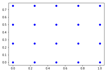
在許多狀況下,我們需要這些格子點來運算,而這些方法可以幫我們快速產生這些格子點。值得注意的是雖然上例的x與y各是5個與4個,但是形成的格子點是4個row及5個column。
-
Talk75_1.py
- 使用fromfunction(function, shape)並根據傳入之function來產生array
- 使用zeros()、ones()、full()、zeros_like()、ones_like()、full_like()等方法來建立值相同之陣列
- 使用empty()或empty_like()來建立無內容之陣列
- 使用indices()與meshgrid()來建立格子點座標陣列
Recap
第七十六話、資料之取得與切片
Numpy的資料取得與陣列類似,但是語法略有不同,如下,首先建立一個二維陣列跟一個2D-array:import numpy as np lista = [[1,2,3],[4,5,6]] arr = np.arange(1,7).reshape(2,3)欲取得陣列中某位置的值,使用如下語法:
print(lista[0][1])若是欲取得nd-array中的值,則語法如下:
print(arr[0,1])除此之外,nd-array允許我們如此取值:
print(arr[[0,1],[1,2]])也就是取得[0,1]與[1,2]兩位置的值,然後將其併為一個array。這樣的方式若是在1D-array也可以使用:
arr1 = np.arange(1, 10) print(arr1) print(arr1[[1,3,6]])取得在arr1中index為1,3,6的元素然後組成一個新的array。所以這樣的形式如果作用在適才的2D-array,則會形成如下情況:
print(arr[[0,1]])取得arr中的index為0與1的元素,分別是row 0與row 1兩個1D-array,然後組合成為一個陣列傳回,因為全部只有兩個row,所以也就是傳回自身。為了方便我們依照類似形式取得陣列中資料,所以numpy允許我們使用切片方式取得資料。Slicing在討論list時已然學過,所以沒甚麼好介紹的,看一下幾個用法,首先建立另一個array:
arr2 = np.arange(15).reshape(3,5)這沒問題,看一下內容:
print(arr2)接下來使用slicing:
print(arr2[:2,1:4:2])x向是:2,也就是0,1(2不包含),而y向則是1:4:2,也就是1,3(步幅為2)。所以得到在index為0的row中、index為1跟3的元素所組合成的一維陣列與index為1的row中、index為1跟3的元素所組合成的一維陣列之組合。
print(arr2[0,:])只有:表示全選,所以得到index為0的row。
print(arr2[:,-1])-1表示最後一個。
print(arr2[arr2>5])取出arr2中所有大於5的元素,組合成一個array。如果僅是arr2>5則傳回一個bool的陣列,大於5者為True。
print(arr2>5)有一點要注意的是使用slicing分割來的陣列並不像分割list一樣會得到一個新的list,只會產生一個新的view,測試一下:
a2 = arr2[0,:] a2[1] = 1000 print(arr2)可見a2只是arr2的一個view(你也可以使用a2.view()方法來得到這個view),修改a2的值也會同時改變arr2,所以若想要有一個新的獨立的陣列,需要使用copy()方法,例如:
print(a2) a2 = arr2[0,:].copy() a2[1] = 1000 print(a2) print(arr2)這樣就可以得到一個新的陣列了。以下兩種語法可以得到跟copy()相同的結果:
a2 = np.copy(arr2[0,:]) a2 = np.array(arr2[0,:], copy=True)上述的copy的預設值就是True。
-
Talk76_1.py
- 使用array[n]取得元素,使用array[[n1,n2]]取得多個元素
- 使用slicing來取得陣列中的部分元素
- 若想得到新的陣列,須使用copy()方法,否則只能得到一個view
Recap
第七十七話、numpy之老生常談
是時候來試試看將numpy用在個例子上,這裡選擇第五十三話的例子。對於於之前每次都重新計算兩點間距離,這次我們先把任兩點距離算出來,儲存到一個array內,之後有需要再取出數值。因為要使用numpy,所以記得要先import,在此還是需要class Node,所以這部分不變。此次在class Route內,加上一個2D-array,用以紀錄任兩點間距離,如下:class Route(object): def __init__(self, nNodes = 20): self.nNodes = nNodes self.nodes = [] self.minLength = None self.minList = None self.arcDistance = np.empty((self.nNodes, self.nNodes)) # <<< self.initializeNodes()這是一個n*n的矩陣,n是所有點個數,因為內容之後會全部更新,所以使用empty()快速產生shape為(n,n)的陣列即可。接下來在初始產生所有點時順便產生所有線段長度:
def initializeNodes(self): """ 初始化所有Node in self.nodes,並計算兩點間距離儲存於self.arcDistance """ rd.seed(20) x = [rd.randint(0, 100) for _ in range(self.nNodes)] y = [rd.randint(0, 100) for _ in range(self.nNodes)] for i in range(len(x)): self.nodes.append(Node(i, x[i], y[i])) for i in self.nodes: # <<< for j in self.nodes: self.arcDistance[i.nodeid, j.nodeid] = self.distance(i, j)因為是一個2D-array,所以使用兩個for loop。然後在計算總長度時,不在每次計算兩點距離,直接自array內讀取即可。
def totalLength(self, route:list)->float: """ 計算儲存在route内的路徑總距離 """ tLen = 0 for i in range(len(route)-1): tLen = tLen + self.arcDistance[route[i].nodeid, route[i+1].nodeid] # <<< # 再加上回程的長度 tLen = tLen + self.arcDistance[route[-1].nodeid, route[0].nodeid] # <<< return tLen剩下的內容原則上都相同,因為有計算執行時間,將會發現如果點數跟執行次數的值不夠大的話,使用array的方式實際上的執行時間會較長,那是因為程式需要先計算任兩點距離一次(使用distance()),反而可能要花更多時間。但是當點數跟執行次數增大之後,使用array的好處便漸漸顯示出來。例如將設定改為
nnodes = 2000 # number of nodes in the problem iteration = 20000 # number of iterations原來做法的計算時間為Time used: 0:01:01.599776,而使用array結構的時間為Time used: 0:00:43.206330。可以看出時間減少了。請自行嘗試使用2D-list來做一次,原則上這樣架構跟array相當,不過array的速度應該更快一些。
第七十八話、numpy運算
當我們有兩個2D-array,我們可能需要做一些計算,numpy允許我們做陣列的運算與矩陣的運算,首先來看陣列的運算。假設我們有以下兩個陣列:x = np.array([[1,3],[5,7]]) y = np.array([[6,8],[2,4]])首先來看四則運算:
print(x+y)相加可以使用+號或是np.add(x,y)。
print(x-y)相減可以使用-號或是np.subtract(x,y)。
print(x*y)相乘可以使用*號或是np.multiply(x,y)。
print(x/y)相除可以使用/號或是np.divide(x,y)。除此之外也可以這樣:
print(x**y) print(x%y)要注意的是以上的運算都是針對兩個陣列的相對位置元素來計算,若是要與數字運算,只要將y換成數字即可,例如:
print(x+1)其他例如x-=1、x*=2、x=x/2、x**=2等運算皆可以。
倘若我們像要進行矩陣運算,則需要呼叫其他函數,例如:
print(x.dot(y)) # or np.dot(x,y)可以使用x.dot(y)或是np.dot(x,y)來計算點積(dot product),請注意x.dot(y)與y.dot(x)並不相同。若是要計算叉積,做法如下:
print(np.cross(x,y))若是要將矩陣轉置,則可使用以下方式:
print(x.T) # or np.transpose(x), or x.transpose()若是要計算內積(inner)與外積(outer)則如下:
print(np.inner(x,y)) print(np.outer(x,y))在許多數學運算中,或許需要反矩陣(inverse),計算反矩陣的方法(inv())放置於線性代數模組(linalg)內,因此可以如此方式取得:
print(np.linalg.inv(x))可以驗算一下,反矩陣與自身的點積會等於單位矩陣:
print(x.dot(np.linalg.inv(x)))
-
Talk78_1.py
- 使用+、-、*、/、**、%等符號來對兩個array進行計算
- 使用dot()、cross()、inner()、outer()來計算點積、叉積、內積、與外積
- 使用np.transpose(x)、x.transpose()、或x.T來計算x的轉置矩陣
- 使用np.linalg.inv(x)來求x的反矩陣
Recap
第七十九話、numpy亂數
在numpy裡面有一個名為random的package,內含許多與隨機數相關之函數,許多部分與之前提過的random模組類似。首先來看如何產生隨機數:print(np.random.random())Package random內的方法random(),可以隨機產生一個0到1之間的實數,你也可以使用random_sample()方法來達到相同的效用。例如:
print(np.random.random_sample())random()方法內的參數size的預設值是None,若是給參數size一個值,則會產生一個包含size個隨機數的array,例如:
arr1 = np.random.random(10) print(arr1)因為產生的是array,所以也可以修改其shape,例如:
print(arr1.reshape(2,5))事實上random.random()方法有一個輸入參數size可以讓我們直接給shape,例如:
print(np.random.random((3,2)))或是
print(np.random.random_sample(size = (3,2)))Numpy還提供另一個較簡便的方法rand()可以直接產生某shape的array,例如:
arr2 = np.random.rand(2,5) print(arr2)要注意rand()的輸入參數是未定長度正整數參數,與random()的tuple並不相同。當然要使用老方法random module也一樣可以得到類似效果:
import random as rd arr3 = np.array([rd.random() for _ in range(10)]).reshape(2,5) print(arr3)顯然看來要形成array還是np.random()來得順暢好用一些。如果想要使用seed()來讓變數變得可以追蹤,可以使用np.random.seed(seed)來設定,例如:
np.random.seed(2019) arr4 = np.random.randint(1,20,12).reshape(3,4)這裡的randint()是用來產生整數亂數的,其中有三個參數,分別為下限、上限、與個數,在例子中也就是要產生1到20間的亂數12個,之後使用reshape()後可以得到:
np.random.seed() # set the seed to be None print(arr4)記得若之後不想讓其他random函數受seed()影響,可以使用np.random.seed()指令來將seed設回None。相同的效果也可以使用直接加上size參數來搞定,如下:
arr5 = np.random.randint(1,20,size = (3,4)) print(arr5)若是要隨機排列,可以使用shuffle()或是permutation(),例如:
temp = list(range(10)) np.random.shuffle(temp) print(temp)Shuffle()會直接(in place)隨機排列原物件(array-like),若是使用permutation()則會傳回新物件,如下:
arr6 = np.random.permutation(temp) print(arr6)若是輸入的array是2D的話,會怎麼隨機排列?
arr7 = np.arange(12).reshape(3,4) np.random.shuffle(arr7) print(arr7)可以看出來僅row被亂排了。除了上述的幾種基本操作之外,random package還提供各種機率分配的數值產生,例如想要產生的數字符合常態分布(Normal distribution),便可使用normal()方法:
print(np.random.normal(0,1,10))此例的輸入參數第一個是平均數,第二個是標準差,第三個是個數(或size)。當然這樣不大看得出來,我們可以先計算所有數字的平均然後與平均數相減來看看是不是很接近來判斷是否合理,當然數字越多越符合,例如:
numbers = np.random.normal(0,1,1000) ave = sum(numbers)/1000.0 print(ave)numbers是根據normal distribution形成的array,長度為1000,據此計算其平均為ave,ave將會很接近0。若是要計算標準差則可以如下方式:
sdsum = 0 for i in numbers: sdsum = sdsum + i**2 sd = (sdsum/1000.0)**0.5 print(sd)結果接近1,所以應該是對的。除此之外,numpy尚提供許多機率分配函數供使用,若有需要可以使用help(np.random)來查詢。
-
Talk79_1.py
- 使用np.random.random()、np.random.random_sample()、np.random.rand()等方法產生隨機實數(0~1),可輸入size參數來給定shape
- 使用np.random.randint()來產生整數亂數
- 使用np. random.shuffle()或np. Random.permutation()來重新亂數排列
- np.random.normal()可產生符合常態分佈的亂數
Recap
第八十話、numpy數學函數
numpy提供各種數學函數供我們計算使用。若上一話的numpy.random類似於python的module random,而此處介紹的數學函數則類似使用了math模組。主要可略分為幾類:- 三角函數
顯然包含sin()、cos()、tan()、arcsin()、arccos()、arctan()等方法,此外還有例如degrees()、radians()、hypot()等,甚至sinh()、cosh()、tanh()之類都是。先看角度與弳度的計算:
d1 = np.degrees([np.pi/6, np.pi/3]) d2 = np.rad2deg([np.pi/6, np.pi/3]) r1 = np.radians([30,60]) r2 = np.deg2rad([30,60]) print(d1,d2,r1,r2)
輸入參數可以為一個數值或是array-like的結構,而rad2deg()與degrees()和deg2rad()與radians()作用相當。接下來看np.sin()的使用:print(np.sin(np.radians(np.linspace(0,90,4)))) print(np.sin(np.radians(30)))
跟math.sin()一樣可以求得sin值,但要特別強調若是math.sin()則參數僅能接受數值,也許我們可以寫一個函數如下:import math def asin(a): if type(a) is float: return math.sin(a) else: for i in a: i = math.sin(i) return a
如此亦可以達到類似效果。其餘的三角函數用法類似,請自行練習。 - 近似值
這包含around()、rint()、fix()、floor()、ceil()、trunc()等,各位應該不陌生,看一下簡單用法:
ra1 = np.random.rand(3,2) print(ra1) rra1 = np.around(ra1, decimals = 2) print(rra1)
跟round()函數一樣求四捨五入值,不過round()僅接受數字,around可以給array-like結構作為參數。Decimals是位數,若是整數位則為0,十位則為-1,例如:ra2 = np.random.randint(1,100, size = (3,2)) print(ra2) rra2 = np.around(ra2, decimals = -1) print(rra2)
其他函數請一樣自行練習。 - 四則運算
原則上計算加減乘除,只是多維的矩陣可根據資料軸來運算,假設有以下兩個陣列:
p1 = np.random.randint(1,10,3) p2 = np.random.randint(1,10,(3,2))
觀察其內的值:print(p1) print(p2)
若是要將其相乘則使用product()方法,例如:print(np.product(p1)) print(np.product(p2))
指定資料軸的話則如下:print(np.product(p2, axis=0)) print(np.product(p2, axis=1))
類似的用法可以用於其他方法,例如:print(np.sum(p2, axis=1))
- 指數與對數
包含exp()、exp2()、log()、log10()、log2()等,跟之前幾類類似,主要是可以用於array-like結構內的所有元素。例如:
e1 = np.random.randint(1,10, (3,2)) exp1 = np.exp(e1)
e1內的所有元素都成為E的次方值,所以exp1內容將為:print(exp1)
若是對其取對數則結果如下:log1 = np.log(exp1) print(log1)
這應該沒有問題。 - 兩矩陣的四則運算
這部分有些已在前面提過,例如add()、substract()、multiply()、與divide()。此外還有reciprocal()、negative()、power()、fmod()、mod()、modf()、remainder()、divmod()等,其中大部分都是關於兩個矩陣的運算,僅與一個矩陣有關的運算為:
re1 = np.reciprocal(e1, dtype = float) print(re1)
此傳回每個元素的倒數,使用dtype指定元素型態為實數。另一個函數modf()的計算如下:mf1 = np.modf(np.reciprocal(e1, dtype=float)) print(mf1)
此函數會分別將小數與整數部分分開傳回。而negative()則只是將陣列乘以-1。print(np.negative(e1))
其他的則與兩個陣列有關,例如我們有兩個矩陣如下:a1 = np.random.randint(1,20,(2,2)) print(a1) a2 = np.random.randint(1,20,(2,2)) print(a2)
試試看power()與mod()來求得次方與餘數:m1 = np.power(a1, a2) print(m1) m2 = np.mod(a1, a2) print(m2)
其餘函數用法類似,請自行練習。 - 其他
其他剩下的例如sqrt()、square()、cbrt()、absolute()等等都算。比方說:
a3 = np.arange(12).reshape(3,4) print(a3) a4 = np.sqrt(a3) print(a4) a5 = np.cbrt(a3) print(a5) a6 = np.square(a3) print(a6)
這三個方法分別會得到平方根、三次方根、以及平方。也可以使用power()方法來得到相同的結果,例如:a7 = np.power(a3, 1/2) print(a7)
此結果與a4相同。而以下結果則與a5相同。a8 = np.power(a3, 1/3) print(a8)
-
Talk80_1.py
- Numpy跟數學相關的內容包括三角函數、四則運算、指數與對數、兩矩陣的四則運算以及其他相關函數
- 此處並無列舉所有方法(例如複數相關函數並無提及),你可由numpy的help()或上網查詢函數列表
Recap
第八十一話、numpy統計函數
在numpy中跟統計有關的函數原則上是常見的基本方法,也可分為幾類如下:- 大小順序
主要是包含min()、max()、ptp()、percentile()等,其用法與build-in-functions又有不同,舉個例子:
a = [[1,2,3],[4,5,6],[7,8,9]] print(min(a))
對於2D-list,應用build-in-function min()所得到的結果是[1,2,3],表示它只能針對該array的第一層內容比較大小,但卻無法針對第一層元素之內的元素比較大小,但是若使用np.min()則如下:print(np.min(a))
它會比較最內層元素然後取得最小。當然這個例子將2D-list改為2D-array結果是相同的。事實上說np.min()除了能夠取得最內層元素的最小,也能夠像min()一樣得到外層array的元素最小,看一下其help():help(np.min)
首先min()與amin()是一樣的,min()只是化名。在輸入參數中可以看到axis,這表示我們可以指定要找哪一軸的最小,例如:print(np.min(a, axis=0)) print(np.min(a, axis=1))
可以看到我們得到x軸與y軸形成的array之最小。順帶介紹另一個方法minimum(),這個方法是比較兩個相同shape的array,然後取得相同位置較小的元素來組合成新的array,例如:大雄=np.array([18, 35, 0]) 胖虎=np.array([25, 12, 10])
這是大雄與胖虎三次小考的成績,請問每一次小考分數較低的分數為何?這樣的問題便可使用minimum()來求:print(np.minimum(大雄,胖虎))
當我們將min()函數應用到不同軸,便可以得到不同的傳回,且與np.amin()得到一樣的結果。再比如ptp()函數會傳回元素範圍,也就是最大減最小的值,例如:k = np.random.randint(1,100,(3,3)) print(k) print(np.ptp(k))
86是92-6得到的。若是要根據個別方向軸,則給參數axis值即可,例如:print(np.ptp(k, axis=1)) print(np.ptp(k, axis=0))
- 平均數與標準差
這大概是印象中最常見的統計了,包含了median()、average()、mean()、std()、var()等。舉例來說,譬如我們有以下的陣列:
a1 = np.random.randint(1,100, size=(3,3)) print(a1)
算一下平均數:mean1 = np.mean(a1) mean2 = np.mean(a1, axis = 0) mean3 = np.mean(a1, axis = 1) print(mean1) print(mean2) print(mean3)
跟之前一樣可以根據不同軸來計算。而average()與mean()的差別在於average()可以給權重,假定每一個row的權重分別是[1,2,3],則可計算如下:ave1 = np.average(a1, axis = 1, weights = [1,2,3]) print(ave1)
標準差跟變異數各位應該沒有問題,例如:std1 = np.std(a1) std2 = np.std(a1, axis = 0) std3 = np.std(a1, axis = 1) print(std1) print(std2) print(std3)
還記得之前測試隨機數是否符合常態分佈的例子嗎?有了標準差函數計算就更容易了。其他部分一樣請自行參照help。在此順道介紹函數apply_along_axis(fun1d, axis, arr),此函數顧名思義就是將某函數應用到某array的某一軸,所以可以這樣做:m0 = np.apply_along_axis(min, axis = 0, arr=a) m1 = np.apply_along_axis(min, axis = 1, arr=a) print(m0) print(m1)
也就是說對於array a的某一軸將min()函數應用上去,此結果於np.min(a, axis=1)與np.min(a, axis=0)結果相同。apply_along_axis()方法內的函數可以自訂,如此我們可以自行建立我們想要的運算,例如:m2 = np.apply_along_axis(lambda x:x+10, axis=0, arr=a) m3 = np.apply_along_axis(lambda x:x**2, axis=0, arr=a) print(m2) print(m3)
當然這些效果都有相應的方法可以使用,但使用這個方法我們可以視需要建立自己的函數來運算。
-
Talk81_1.py
- 使用min()、max()、ptp()、percentile()等來得到數值的大小或比例
- 使用median()、average()、mean()、std()、var()等來得到平均數或標準差
- apply_along_axis(fun1d, axis, arr)函數可讓我們使用自訂函數應用到矩陣計算
Recap
第八十二話、陣列的分分合合
之前提過陣列可以使用slicing,但是只是一個view,並不是真的改變陣列的型態,若要改變一個array的陣型,可以直接修改其shape或是使用reshape()方法。那若是要將一個array拆成兩個呢?首先先建立一個array:arr1 = np.random.randint(1,100, (4,4)) print(arr1)接下來要分拆陣列,使用np.hsplit(ary, indices_or_sections)方法:
arr2 = np.hsplit(arr1, [2,]) print(arr2[0]) print(arr2[1])hsplit是分拆horizontal方向,[2,]的意思是將前兩個column分成一組,剩下其他的分為一組。若是要分拆vertical方向,則可以使用vsplit(),例如:
v1, v2 = np.vsplit(arr1, [2,]) print(v1) print(v2)如果要切分超過兩個,可以如下:
arr4 = np.vsplit(arr1, (1,2,)) print(arr4)(1,2,)這個意思就是把第一個row1做第一份,row2做第二份,剩餘全部的當作第三份。也可以直接使用split()這個方法,再在裡面的參數axis設定方向即可(axis預設值為0),例如:
arr5 = np.split(arr1, (2,), axis = 1) print(arr5)跟hsplit()的效果一樣。另一個拆分方法是array_split(ary, indices_or_sections, axis=0),這個方法會直接幫我們把array平分為數份,若是無法均分也不會傳回錯誤,還是會將array分為大小接近的幾份,例如:
arr6 = np.array_split(arr1, 3, axis=0) print(arr6)分為三份,因為無法等分,變成2,1,1。切分axis=0或1這兩軸現在應該沒有問題,不過若是有三軸的時候怎麼辦?此時可以使用dsplit()方法,例如:
arr7 = np.random.randint(1,100, (2,2,2)) print(arr7)先設計一個3D-array,然後使用dsplit()如下:
print(np.dsplit(arr7, (1,)))原則上也可以使用split(axis=2)來達到一樣效果,例如:
print(np.split(arr7, (1,), axis=2))了解了拆分,接下來看如何組合兩個array。首先我們回顧一下如果是兩個list相加,可以結合兩個list,如下:
lista = [1,2,3] listb = [4,5,6] print(lista+listb) listc = [[1,2],[3,4]] listd = [[5,6],[7,8]] print(listc+listd)不過如果是兩個array用+號連結,結果會是個別元素相加,各位應該還記得。舉個簡單的例子:
print(np.array([1,2])+np.array([3,4]))所以如果要把兩個array組合成一個,需要使用方法hstack或vstack。首先先建立兩個陣列:
x = np.arange(4).reshape(2,2) y = np.arange(100,104).reshape(2,2)因為兩個的shape都是(2,2),所以從哪一個方向來組合都OK,如下:
arr8 = np.vstack((x,y)) print(arr8)再試另一個方向:
arr9 = np.hstack((x,y)) print(arr9)要注意其中的參數是一個tuple,因為只接受一個參數。此外,如果要組合的方向行或列數量不同,則會傳回錯誤。那有沒有像split()類似的方法稱為stack()呢?其實是有的,不過效果並不相同,使用stack()會從一個新的軸疊加,而不是組合成一個陣列,甚麼意思呢?例如:
arr10 = np.stack((x,y), axis=0) print(arr10)這是將兩個陣列從另一個軸疊加兩個陣列,而不是跟np.vstack()一樣將兩個陣列順著某一軸合併成一個陣列。此外,使用v與h來分辨方向有時候可能比較混淆,使用另兩個相同內容的方法或許比較容易理解:
arr11 = np.row_stack((x,y)) arr12 = np.column_stack((x,y)) print(arr11) print(arr12)再者,雖然stack()的意思不同,其實還是有一個與vstack()和hstack()意思相同的方法且可以指定參數axis方向的,那就是concatenate():
arr13 = np.concatenate((x,y)) print(arr13) arr14 = np.concatenate((x,y), axis=1) print(arr14)這個方法有一個特殊點就是將axis設為None:
arr15 = np.concatenate((x,y), axis=None) print(arr15)有時候我們會需要將所有內容攤平成為1D-array,方便我們操作陣列。不過要將內容攤平成1D-array,有較方便的方法便是使用flatten()或是ravel(),例如:
arr16 = np.concatenate((x,y)).flatten() print(arr16) print(np.concatenate((x,y)).ravel())其實我們也可以藉由修改array的shape來將其攤平,例如:
arr17 = np.concatenate((x,y)) arr17.shape=(8) print(arr17)要注意的是不能使用reshape(1,8),因為這樣會形成如下的array:
arr18 = arr17.reshape(1,8) print(arr18)可以看出來其實我們期待的是arr18[0]。可以想見如果我們想要traverse array中的個別元素,或是譬如要得到所有元素之和,可以先將array的元素攤平然後使用一個for loop搞定,否則就得使用兩個for loop,顯然一個應該容易多了,使用arr1試試看:
s = 0 for e in arr1.ravel(): s += e print(s)當然因為我們已經學會數學函數,所以這個結果可以用np.sum(arr1)來取得更快。
-
Talk82_1.py
- 欲拆分一個array,可以使用np.hsplit()、np.vsplit()、np.split()等方法,若欲拆分第三軸,則可以使用np.dsplit()或np.split(axis=2)
- 欲組合兩個array,可以使用np.hstack()、np.vstack()、np.row_stack()、np.column_stack()、np.concatenate()等,若是使用np.stack()則往第三軸疊加
- 欲攤平一個array,可以使用flatten()或ravel()方法
Recap
第八十三話、陣列與檔案
numpy提供方便的函數讓我們可以跟檔案溝通,讓陣列的內容可以很容易的儲存到檔案內,或是自檔案取得資料。先看如何儲存資料,製作一個陣列如下:import numpy as np np.random.seed(2019) arr1 = np.random.randint(1,100, size=(5,5))若要將arr1存入到一個檔案,直接使用save()方法,如下:
np.save('npsave1', arr1)有這個指令,便會將陣列arr1存入npsave1這個檔案內,其延伸檔名為.npy。若是要將其內容讀出,則使用load()方法,例如:
np.load('npsave1.npy')這樣我們便可以將陣列的資料內容利用檔案傳遞。不過如果我們試著用記事本打開npsave1.npy這個檔案,會看到一些看不懂的亂碼,畢竟npy這樣的延伸檔名並不是文字檔。所以若要儲存為文字檔,則可以使用savetxt()與loadtxt()兩個方法,例如:
np.savetxt('npsave2.txt', arr1)此時打開npsave2.txt這個檔案,會看到內容格式是使用科學記號。看一下help:
help(np.savetxt)若是要改變儲存格式,則改變其參數fmt,例如:
np.savetxt('npsave2.txt', arr1, fmt='%d')使用d(decimal)或i(integer)表示是整數,若是f(float)表示是實數,例如fmt=’%.2f’表示到小數後兩位。預設值%.18e表示小數後18位的科學記號。若是字元則使用c(character),字串則使用s(string)。再者,delimiter=’ ‘表示資料內容使用一個空白區分,若是要使用其他符號例如逗點,則可更改為delimiter=',',如此顯示的資料便會使用逗點區分,例如:
np.savetxt('npsave2.txt', arr1, fmt='%i', delimiter=",")請打開檔案看結果。若是要讀取內容,使用loadtxt()方法,先看一下help:
help(np.loadtxt)因為剛剛的檔案內容是使用逗點做delimiter,所以讀取的時候也是要使用一樣的delimiter,於是:
np.loadtxt('npsave2.txt', delimiter=',')如果使用的是delimiter為一個空白,則delimiter可使用預設值。若是想要改變內容資料的資料型態,則修改dtype,例如:
np.loadtxt('npsave2.txt', dtype=int)這樣是不是很容易?若是使用之前學過的檔案存取方式,需要使用如下的做法:
with open('npsave3.txt', 'w') as f: for line in arr1: for data in line: f.write(f"{data} ") f.write('\n')不可以直接將line寫進去檔案,因為line會是一個array,則會變成好幾個array。若是要讀出資料則如下:
arr = [] with open('npsave3.txt', 'r') as f: for line in arr1: arr.append(line) arr2 = np.array(arr)因為讀出來又要變成另一個nd-array,所以需要經過這些步驟,比之loadtxt()這樣的方法當然是麻煩很多了。另一個狀況是如果有一個檔案(.txt或.csv)如下:
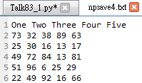
這個資料有一行標頭(title),不過這行是我們不需要的內容,而且如果直接讀取此檔案(npsave4.txt),會讀到文字與數字,若要使用數字還需要將其自文字轉換為數字。這種情況的話,若要讀取資料則可以使用genfromtxt()這個方法,看一下help:
help(np.genfromtxt)有點長,前面幾項跟之前的方法類似,直接使用試試看:
arr3 = np.genfromtxt('npsave4.txt') print(arr3)Oops! 第一行的文字變成了nan(not a number),那若是將資料型態改為文字呢?
arr4 = np.genfromtxt('npsave4.txt', dtype=str) print(arr4)這樣雖然可以得到所有內容,不過要記得之後若要使用數字必須將得到的內容cast為數字。再者,反正不需要標頭這一行,直接捨去算了,此使採用參數skip_header=1:
arr5 = np.genfromtxt('npsave4.txt', skip_header=1) print(arr5)直接跳過第一行。這是個方便的指令,例如我們想要跳過前面三行,只要將skip_header=3即可。除此之外,尚可以使用usecols這個參數來強調僅取用某幾個column,例如:
arr6 = np.genfromtxt('npsave4.txt', usecols=(1,2), skip_header=1) print(arr6)當然其實重點在將陣列讀入,只要有了整個陣列,僅需要使用切片(slicing)即可得到陣列的任何部位了。上述的檔案讀取都僅限於一個陣列,若是現在有超過一個陣列要儲存到檔案內要怎麼辦?有幾個陣列做幾個檔案嗎?當然不是。此時可以使用另一個儲存方法稱為savez(file, *args, **kwds),這個方法可以讓我們把多個陣列儲存到一個延伸檔名為npz的檔案內。例如我們有以下幾個陣列:
a1 = np.array([['a','b','c'],['d','e','f'],['g','h','i']]) a2 = np.arange(12).reshape(3,4) a3 = np.random.randint(1,100, (5,5)) a4 = np.sqrt(a3)接下來要將這些陣列存入檔案npsave5中:
np.savez('npsave5', a1, a2, ran = a3, sqr = a4)這行指令表示將a1~a4儲存到npsave5.npz這個檔案內,其中a3與a4給了名稱分別為ran與sqr。現在有了npsave5.npz這個檔案,我們使用load()方法來開啟並取得其中的陣列:
arrs = np.load('npsave5.npz')此時可以先查看npsave5.npz之中有幾個陣列:
print(arrs.files)可以看出其中包含了我們適才命名的ran與sqr,還有兩個arr_0與arr_1,這兩個分別代表a1與a2,因為一開始沒有給名稱,所以程式便自動幫我們建立名稱。現在可以取得其內的陣列:
print(arrs['arr_0']) print(arrs['ran'])利用這方式,我們可以將多個陣列儲存到一個檔案中。
-
Talk83_1.py
- 使用save()與load()方法來讀取檔案內的陣列
- 使用savetxt()與loadtxt()方法來讀取檔案內的陣列,此時檔案為文字檔
- 使用np.genfromtxt()方法來取得文字檔內容,並可以使用參數來控制讀取哪部分的陣列
- 使用np.savez()方法來儲存多個陣列到一個檔案
Recap
第八十四話、陣列排序
根據之前提過的,排列大小是我們可能常需要做的事情。如果我們使用sorted()排序二維list,則會如下:lista = [[5,7,3],[7,4,7],[1,3,2]] print(sorted(lista))不過此方法卻無法幫我們排序陣列,例如:
k = np.array(lista) print(sorted(k))Sorted()無法排序陣列其實是不完全正確的,因為若是1D-array其實是可以的,例如:
print(sorted(np.random.randint(1,100,10)))當然現在我們在乎的是如何排序2D-array,而欲排序一個二維陣列,可以使用np.sort()方法,看一下help:
help(np.sort)馬上試試看:
np.random.seed(84) k = np.random.randint(1,100,(3,2)) print(np.sort(k))這跟sorted()排序二維list的結果是截然不同的,使用sorted()並不會影響每一個row之中的list內元素的順序,而是將list內的每個元素拿來排序,只是前例的元素也是list罷了。而且list排定大小只是比較第一個元素,其內的其他元素順序並不受影響。而np.sort()則是針對某一軸的元素做排序,所以得到的結果並不相同。再次驗證,這次使用np.sort()來排序lista如下:
print(np.sort(lista))其內的list元素中的數字被排序了(數字順序改變)。之前的例子使用預設值axis=-1,表示使用最後一軸,若是使用其他軸,例如:
print(np.sort(k, axis = 0))column方向的元素被排序了。如果陣列中的元素不只是數字,而是一個物件,那排序的結果會如何?我們之前提過若是要比較兩個物件大小,需要設計物件比較大小的方法,在此我們只要給定要根據那個屬性來排序即可,舉個例子:
from collections import namedtuple ranking = namedtuple('ranking', ['name', 'math','eng'])使用之前介紹過的namedtuple來設計一個簡單的學生成績物件,接著建立幾個物件:
s1 = ranking(name = 'Tom', math = 10, eng = 5) s2 = ranking(name = 'Mary', math = 30, eng = 15) s3 = ranking(name = 'John', math = 60, eng = 55) s4 = ranking(name = 'Allen', math = 60, eng = 65) s5 = ranking(name = 'Hellen', math = 100, eng = 100) s6 = ranking(name = 'Steve', math = 50, eng = 70)現在再設計一個資料型態的list如下:
dt = [('name','S10'), ('math',int), ('eng',int)]這是每個物件的資料型態,之後會根據這些型態來排序。將上列物件存入一個list內,如下:
students = np.array([s1,s2,s3,s4,s5,s6], dtype = dt)現在可以根據每個物件的某一屬性來排序,例如根據數學:
print(np.sort(students, order='math'))若是數學相同者,再根據英文排序,則直接給兩個屬性如下:
print(np.sort(students, order=['math', 'eng']))至於排序的演算法,無論是quicksort或是mergesort則不在此處討論。如果上例的成績是儲存在兩個不同的array,那麼是否可以得到相同的結果?當然是可以,此時可以使用另一個排序方法稱為lexsort(),舉例如下,首先將上述資料整理成如下:
name = np.array(['Tom','Mary','John','Allen','Hellen','Steve']) math = [10,30,60,60,100,50] eng = [5,15,55,65,100,70]接下來使用lexsort():
sindex = np.lexsort((name, eng, math)) for i in sindex: print(f"({name[i]},{math[i]},{eng[i]})", end='')首先看一下sindex的內容:
print(sindex)這個array內的資料是math排序後的對應index,也就是說如果我們取得對應在math的對應位置資料會得到排序後的數列,看一下上述的for loop印出來的結果:
(Tom,10,5)(Mary,30,15)(Steve,50,70)(John,60,55)(Allen,60,65)(Hellen,100,100)
此結果與之前的相同。也就是說,當我們傳入參數(name,eng,math)進入lexsort(),lexsort()會首先根據math進行排序,若是math中有相同資料,則根據eng再度排序,若是兩者皆相同,則再根據name排序,而傳回的是對應的索引值(index)。其實還有另一個方法可以得到排序數值對應的index排列,那就是argsort()方法。例如:
arr1 = np.random.randint(1,100,5) print(arr1)使用argsort()方法:
arg = np.argsort(arr1) print(arg)得到的是index的array,取得對應的值如下:
print(arr1[arg])如此可以得到值的排序。不過這與lextsort()不同,僅針對一個array做排序。
若是我們想將物件分群,譬如說取得分數最低的3個,我們當然可以先排序再得到前3個數字,若是不在乎取得的數值是否排序好,那麼我們可以使用partition()方法,例如有如下的數據:
arr2 = np.random.randint(1,100,10) print(arr2)使用partition()方法分群:
arr3 = np.partition(arr2, 2)這個例子的意思是把最小的兩個值挪到左邊,剩下的值移往右邊,但是不保證他們的排序,例如:
print(np.partition(arr2,7))把前面較小的7個數移到左邊,但是並不一定排序。若是要分為三群,可以將參數改為如下:
print(np.partition(arr2,(2,7)))左邊是最小的兩個數,右邊是比第7小還大的數,中間則是介於第2小跟第7小的數字。跟之前的sort()與argsort()類似,partition()有一對應方法argpartition()可以得到partition後的對應index,例如:
arg = np.argpartition(arr2, 2) print(arg)將arg套入arr2,可以得到partition的結果如下:
print(arr2[arg])
-
Talk84_1.py
- 使用np.sort()方法來排序陣列,給定order參數可以排序有結構的物件
- 使用np.lexsort()方法來排序多個陣列
- 使用np.argsort()來得到排序後之對應index
- 使用partition()來將數值分群,argpartition()則回傳分群後的對應index
Recap
第八十五話、閒聊陣列
Numpy的基本觀念談得差不多了,在此做一些補充。- Broadcast
之前提到許多陣列間的運算例如加減乘除,直覺都認為兩個陣列需shape相同,事實上並不需要,例如:
x = np.array([1,2,3]) y = np.array([[1,2,3],[4,5,6]]) print(x+y)
又如:print(x*y)
此稱之為Broadcast,可以看出來在運算時x自動往y的較長方向延伸計算。又或者是:w = np.array([[1],[2]]) print(y) print(w+y)
w也會自動往y的較長方向延伸計算。不過如果連一邊的shape都不能對應,則會出現錯誤。例如:z = np.array([1,2]) print(y) print(z+y)
- nditer()與flat
之前提過若想要使用for loop來traverse整個陣列,可以先使用ravel()或是flatten()攤平陣列,然後便可以從頭到尾一個一個取得資料。不過若是要得到iterator,則可以使用nditer:
k = np.random.randint(1,100, (3,2)) print(k) for i in np.nditer(k): print(i, end=" ")
若是要改變traverse的順序為fortran like,則可以直接修改參數order為’F’即可。for i in np.nditer(k, order='F'): print(i, end=" ")
不過事實上這個order參數ravel()與flatten()也都有,如下:for i in k.flatten(order='F'): print(i, end=" ")
或是如下:for i in np.ravel(k, order='F'): print(i, end=" ")
當然這些都不是回傳一個iterator,而是一個陣列。除了使用nditer()方法來得到iterator之外,也可以使用flat來取得一個iterator 物件,例如:for i in k.flat: print(i, end=" ")
flat跟flatten()的分別是flat傳回一個iterator,而flatten()則是傳回一個攤平後的陣列copy。不過flat倒是沒有order=’F’的選項。 - where() & extract()
where()方法可以讓我們擷取陣列中符合某條件的資料,譬如說我們有以下的陣列:
w1 = np.random.randint(1,100, 10) print(w1)
現在如果我們想要找出大於50的資料,則可以使用where()如下:ind = np.where(w1>50) print(f"大於50的值:{w1[ind]}")
where()傳回的是索引值(index),所以再放回w1得到值。如果是2D-array的話呢?先設計個2D-array如下:w2 = np.random.randint(1,100,(3,3)) print(w2)
接下來得到符合條件的數值之index:ind2 = np.where(w2>50) print(ind2)
因為是2D-array,所以得到兩組數字分別代表第一軸跟第二軸,可以使用以下方式來得到大於50的值:for i,j in zip(ind2[0], ind2[1]): print(w2[i][j], end=" ")
當然你也可以寫這樣:print([w2[i][j] for i,j in zip(ind2[0], ind2[1])])
如果不想經過先取得索引值的步驟,則可以直接使用extract()來得到想要的結果,例如:print(f"大於50的數:{np.extract(w2>50, w2)}")
要記得extract()需要兩個參數,一個條件跟一個陣列本體。再試一次,這次找出w2中三的倍數:print(f"三的倍數:{np.extract(np.mod(w2, 3)==0, w2)}")
- 線性代數
學了numpy,原則上學會了陣列的建立與操作。這些矩陣可以協助我們求解許多相關的數學問題,例如在linalg這個package內便包含許多相關的線性規劃公式函數。譬如說有以下的聯立方程組:
3x - 5y = 10
使用np.linalg.solve()方法可以直接求解,如下:
2x + 3y = 13a = np.array([[3,-5],[2,3]]) b = np.array([10,13]) ans = np.linalg.solve(a,b) print(ans)
是不是變得很容易?又或者要計算矩陣的行列式,可以使用如下方式:arr1 = np.array([[1,2],[3,4]]) print(np.linalg.det(arr1))
如果需要做數學的求解或計算以及資料分析,numpy和scipy等確實是強大的工具。
-
Talk85_1.py
- BroadCast性質讓我們可以計算不同形狀的陣列
- nditer()與flat會傳回iterator
- 可利用where()與extract()函數來得到符合某條件的陣列元素
- 使用np.linalg中的函數可求解線性代數問題
Recap
Python亂談
熊貓
第八十六話、熊貓
熊貓(Pandas)是Python中的另一個處理套件,主要的資料結構可以分為Series與Data Frame兩種。欲使用熊貓內之資料結構與方法,顯然需先import pandas,所以先以如下方法建立一個series:import numpy as np import pandas as pd ser1 = pd.Series(np.arange(5))首先導入pandas兩個package,然後使用Series()方法來建立一個series,傳入參數可以是list、tuple、dict、array,因為numpy的資料結構可以輕易的嵌入在pandas的資料結構內互相套用,所以通常會一起使用。看一下ser1內容:
print(ser1)可以看到有兩行資料,其中第一行稱為索引值(index),第二行則為數值(value)。Value是我們的資料,index是要讓我們得到資料的索引。所以如果說numpy的array結構是類似list的結構,那麼Pandas的Series與Data Frame結構或許可說是類似dict的結構。現在試著使用index來取得其中的值,例如:
print(ser1[1])Dict與list的不同處便是dict可以使用自訂的索引來處理資料,而Series與array的差別也是類似,所以現在我們再建立另一個series看看:
ser2 = pd.Series([2,4,6,8,10], index=['a','b','c','d','e']) print(ser2['c'])我們將這個例子中ser2的index設定為字元,根據其索引值可以得到ser2[‘c’]為6,而ser2的內容如下:
print(ser2)現在可以明顯看出series與list或array的區別,也解釋為何說series比較像是一個dict,因為其中的數值可以使用自訂的index來取得而不像array或list僅能使用內定的編號來取得資訊。雖然或許使用numpy array或list可以達到相同結果,在某一方面series就像dict讓我們更容易明白操作的內容,例如:
eng = {"大雄":0, "小杉":100, "胖虎":30, "靜香":80, "小夫":60} ser3 = pd.Series(eng)eng為英文考試成績,我們可以將此dict傳入pd.Series()內,此時我們可以得到ser3的內容如下:
print(ser3)我們一樣可以如此得到資料:
print(ser3["小杉"])用法跟dict好像一樣。不過Series與array一樣,其中的資料型態都是相同的,此點與dict並不相同。Series是Pandas的基本型態,若說Series是1D-array,那個DataFrame便是2D-array了,事實上DataFrame就是多個Series的組合,宣告的時候使用方法DataFrame(),例如:
df1 = pd.DataFrame(np.arange(12).reshape(3,4)) print(df1)傳入參數可以是2D-array、2D-list、或是dict。很明顯可以看出這個data frame是由4個series組成,每個series有3筆資料,索引值為0、1、2。我們可以使用以下方式得到其中資料:
print(df1[3][1])要注意的是第一個索引指的是編號為3這個series,然後1視為其中index為1的資料,跟2D-array的資料取得方式不同。現在再建立另一個data frame來加深了解。首先假設我們有一個如下的2D-list:
list2 = [[1,2,3],[4,5,6],[7,8,9]]將此2D-list作為傳入參數來建立data frame:
df2 = pd.DataFrame(list2, index = ['A','B','C'], columns = ['One','Two','Three']) print(df2)其中columns參數就是每一個Series的名稱,而index參數就是Series內的索引值。所以我們欲取得資料需要這樣做:
print(df2['Two']['C'])事實上只是先取得某一個series,然後取得在series內某一索引值的資料。我們已經知道series與data frame內的資料會有相同的資料型態,現在來看看它們的其他屬性。
- 軸的(axes)屬性
首先是軸的(axes)屬性,也就是紀錄index與columns的內容,例如:
print(ser2.axes)
或是print(df2.axes)
不過對我們來說這些axes已經有固定名稱了,也就是index與columns,所以也可以如此取得軸資訊:print(ser2.index)
或是print(df2.index) print(df2.columns)
我們甚至可以直接修改這些值來改變其index,例如:ser1.index = ['a','b','c','d','e'] print(ser1)
columns也可以使用相同的方式來修改。 - 資料型態(dtype、dtypes)
Series內的資料有相同的資料型態,紀錄在dtype或dtypes參數。若是Data Frame則僅能使用dtypes參數,例如:
print(ser2.dtype) print(df2.dtypes)
那麼如果我們要將不同資料型態的資料加入會發生甚麼事?如下:ser2['b'] = 3.14159 print(ser2)
可以發現即使指派了float,還是讓其變成了int64。再看看data frame:df2['Two']['B'] = 3.14159 print(df2)
跟series一樣,還是變成了int。不過如果我們這樣做:df2['Two']['B'] = "3.14159" print(df2)
怪了,資料顯示不同了。看一下其dtypes:print(df2.dtypes)
編號為Two的Series資料型態變成object了,也就是說此資料無法轉換成int,所以為了資料型態都相同,所以將此series的資料型態自動修正為object。那麼若是我們自己想要修改資料型態呢?我們是不可以直接設定dtype的值的,不過可以使用astype()這個方法,例如:ser1.astype(float)
若要改變data frame內某一個series的值,可以使用相同的操作,例如:df2['Two'].astypes(float)
順道一提,如果要計數一個DataFrame中的dtype各有多少,可以使用get_dtype_counts()方法來求得。 - 資料大小
儲存不同類型資料型態顯然影響記憶體使用,我們可以使用itemsize參數來觀察其資料大小,例如:
print(ser1.itemsize)
因為ser1的dtype是int32,表示儲存一筆資料使用32個bits,也就是4個bytes。print(df2['Two'].dtypes) print(df2['Two'].itemsize)
df2[‘two’]的dtype是物件,其itemsize是8個bytes。若要知道整個架構所使用的記憶體,則將itemsize乘以資料總筆數,或是使用nbytes參數,如下:ser1.nbytes ser1.itemsize*ser1.size
Data frame並沒有nbytes這個參數,若要計算可以將其拆分為一個一個Series分開計算即可。而size參數記錄著series的資料總個數,例如:print(df1.size)
事實上就是其index與columns個數的乘積,也就是其shape,可由shape參數得知,例如:print(df1.shape)
-
Talk86_1.py
- 使用pandas的series與data frame需先import pandas
- 宣告series與data frame可以傳入list、tuple、dict、array等資料結構
- 取得或改變軸的內容可以使用index、columns參數
- 可以使用dtype(dtypes)來查看資料型態,若要改變型態則可以使用astype()方法
- 在series中使用itemsize來查看一筆資料的大小,使用nbytes來得到所有資料佔記憶體的大小
Recap
第八十七話、熊貓資料選取與修改
上一話提及Series類似dict,若要取得其中資訊可直接使用index來找到對應值,例如以下的Series:import numpy as np import pandas as pd ser1 = pd.Series(np.arange(5), index=['a','b','c','d','e'])取得其中資料的方式:
print(ser1['a'])逐個取得資料的方式:
for i in ser1.index: print(f"{i} => {ser1[i]}")而DataFrame則是多個Series的組合,所以只要先取得一個Series然後再根據Series的資料取得方式得到資料即可,例如如下的DataFrame:
df1 = pd.DataFrame(np.random.randint(1,100,(3,3)), index = ['a','b','c'], columns = ['one','two','three'])取得資料方式如下:
print(df1) print(df1['two']['c'])其中df1[‘two’]其實就是取得two這個series。如果我們堅持要使用數字數列的編號來取得資料,可以使用iloc,例如:
print(ser1.iloc[0])這個ser1[‘a’]的結果是一樣的。也可以如下使用:
print(ser1.iloc[1:3])選擇切片。或是
print(ser1.iloc[[1,3,4]])選擇多個特定位置。或是
print(ser1.iloc[[True,False,True,True,False]])選擇True的位置。當然也能用於dataframe,例如:
print(df1.iloc[2][1])這裡要特別注意的是如果使用iloc,表示第一個參數指標是row,第二個參數指標是column,且編號是由0開始,與剛才的先取得Series再找到index位置的做法是顛倒的。相對於取得一個Series的方式,iloc主要是讓我們可以得到一個row,也就是取得在所有Series中相同index的資料。舉例來說,譬如我們建立以下的dataframe:
df2 = pd.DataFrame(np.random.randint(1,100,(3,3)), index = ['desk', 'pen', 'computer'], columns = ['class A', 'class B', 'class C'])其內容是三個班級所擁有的設備數量:
print(df2)我們可以很容易的得到某一班的設備數,若想知道每班的電腦數,則使用iloc:
print(df2.iloc[2])當然若要使用切片或使選擇多個row也是沒問題的,如下:
print(df2.iloc[0:2]) print(df2.iloc[[0,2]])當然也可以置入一個True-False的list來取得對應的row,請自行嘗試以下取法:
print(df2.iloc[0:2, 0:2]) print(df2.iloc[[True,False,True]])為了讓取得row這個步驟更加像dict,應該要捨棄使用從0開始的數列index,直接使用定義的index,這樣的方式為loc,例如:
print(ser1.loc['c'])loc的切片與iloc的定義稍有不同,例如:
print(ser1.loc['a':'c'])注意index=’c’的資料也被選取了。用在data frame的做法類似,例如:
print(df2.loc['pen':'computer','class B':'class C'])或是
print(df2.loc[['pen','desk'],'class B':'class C'])也請嘗試以下的取得方式:
print(df2.loc['pen']) print(df2.loc[df2['class A'] > 30]) print(df2.loc[lambda df: ['pen', 'computer']]) print(df2.loc[ [True,False,True], [False,True,True] ]) print(df2[1:3]) print(df1['c':'k'])這個方式可以同時有iloc與loc的特性。若是僅要取得一個元素,也可以使用at與iat來取得資料,例如:
print(df2.at['pen', 'class C']) print(df2.iat[1, 2])在定義DataFrame的columns,名稱最好不要有空白,像上例中的class A算是不好的示範,因為我們可以如此取得一個Series:
print(df1.one)你可以想像如果輸入
df2.class A會產生怎樣的錯誤。
當我們要改變Series或是DataFrame內的資料時,一樣使用取得資料的方式,然後將值指派給該位置即可,例如:
df2.at['pen','class C'] = 100 print(df2)這應該沒有問題,若是選擇的元素超過一個時則如下:
df1.loc['a'] = [1,2,3] print(df1)或是如下:
df1.loc['a':'b', 'one':'two'] = [[1,2],[3,4]] print(df1)根據之前提過的Broadcast原理,我們若僅給一個值,則所有被選擇的元素都會變成該值,例如:
df2.iloc[1] = 10 print(df2)或是
df2.iloc[:2, :2] = 0 print(df2)
-
Talk87_1.py
- 使用dataframe[‘seriesname’]自DataFrame取得一個Series
- 使用iloc與loc來取得相同index之row
- 使用at與iat來取得單一元素
- 定義columns時,名稱最好不要有空白
Recap
第八十八話、熊貓的indexing
我們已經知道在熊貓的data frame中,每一行稱之為index,每一列稱之為columns,而事實上我們可以分別給它們一個總稱,稱為index name與columns name,例如假定有以下的一個DataFrame:import numpy as np import pandas as pd np.random.seed(1) df1 = pd.DataFrame(np.random.randint(1,100,(6,3)), index = ['a','b','c','d','e','f'], columns = ['key','pen','desk']) np.random.seed(None)設定其index name與column name可直接使用以下方式:
df1.index.name = "class" df1.columns.name = "item" print(df1)而若想修改index與columns的內容,可以透過rename(index=None, columns=None, **kwargs)方法,例如:
df1 = df1.rename({'a':'A', 'c':'C'}, {'pen':'pencil'}) print(df1)使用兩個mapper來修正index與columns內容,若是僅想修正某一軸,則直接傳入某一mapper即可。當然也可以如第八十六話中所述,使用
df1.index = ['a','b','c','d','e','f'] print(df1)來修改index內容。除此之外,也可以使用rename_axis(mapper, axis=0, copy=True, inplace=False)方法來修改軸(index與columns)名稱,例如:
df1 = df1.rename_axis({'a':101,'b':102,'c':103}, axis = 0) print(df1) df1 = df1.rename_axis({'pencil':'marker'}, axis = 1) print(df1)其中axis的預設值為0,也就是說要使用rename_axis()來修改columns的名稱必須要給定axis=1。事實上也可以使用set_axis(axis, labels)方法來直接修改軸名稱,例如:
df1.set_axis(0,[1,2,3,4,5,6]) df1.set_axis(1,['key','pen','desk']) print(df1)數字序列可以使用range(1,7),原則上此方式等同於設定df1.index與df1.columns。
如果說我們想要針對每個column的名稱加上字首或字尾,則可以使用add_prefix(prefix)或是add_suffix(suffix)方法,例如:
df1 = df1.add_prefix("item_") df1 = df1.add_suffix("_") print(df1)此方法若是應用在Series,則修改的是index。不過若是想要修改DataFrame的index要怎麼辦?可以採用如下方式:
df1 = df1.rename("class_{}".format) print(df1)或是使用以下方法也可以:
df1.index = df1.index.astype(str)+"_class" print(df1)若是我們想要重新排列index的順序,可以使用reindex(index=None, columns=None, **kwargs)方法,例如:
df1.set_axis(0,range(1,7)) df1 = df1.reindex([1,3,6,2,5,4]) print(df1)Set_axis()只是將index改為序列,方便做reindex()。若是想要將row隨機排列,可以使用如下方式:
df1.index = ['a','b','c','d','e','f'] index1 = list(df1.index.copy()) np.random.shuffle(index1) df1 = df1.reindex(index1) print(df1)我們可以針對Series進行shuffle,不過對於DataFrame內的Series可能會出現錯誤,因為僅有該Series被打亂排列。事實上我們還可以讓DataFrame中的某一行或某一列成為columns或index的名稱,只要使用set_index(keys, drop=True, append=False, inplace=False, verify_integrity=False)方法,例如:
df1 = df1.set_index("key") print(df1) df1 = df1.set_index(['key','desk']) print(df1) df1 = df1.set_index(['key',[0,1,2,0,1,2]]) print(df1)上述的df1.set_index([‘key’,’desk’])是將此二Series當作index,又稱為多重index。如果想要回復原來的index,可以使用reset_index()方法,不過回復後的index會變成數列,所以若想要原來的index需重新設定,如下:
df1 = df1.reset_index(level=0) print(df1) df1.index = ['a','b','c','d','e','f'] print(df1)最後介紹stack()與unstack()來將DataFrame轉換成多重index,例如:
df1.index = ['a','b','c','d','e','f'] df1.columns = ['key','pen','desk'] df1 = df1.stack() print(df1) df1 = df1.unstack() print(df1)也就是使用stack()後,index與column合併為多重index,再使用unstack()會回復原樣。
-
Talk88_1.py
- 使用index.name與columns.name來定義index與columns的名稱
- 使用rename()或reanme_axis()或set_axis()來修改index或columns的內容
- 使用add_prefix()或add_suffix()來增加DataFrame的column name或是Series的index name的字首或字尾,至於DataFrame的index則請參考文內敘述
- 使用reindex()來重新排列row的順序、使用set_index()來使用內容資料當作index
- 使用stack()來建立多重index,並使用unstack()來去除多重index
Recap
第八十九話、再話資料選取
接續前一話,來看看其他的資料選取方式。使用上一話的df1,若是我們想要得到前幾個或後幾個row,可以使用head(n=5)與tail(n=5)函數,例如:import numpy as np import pandas as pd np.random.seed(1) df1 = pd.DataFrame(np.random.randint(1,100,(6,3)), index = ['a','b','c','d','e','f'], columns = ['key','pen','desk']) np.random.seed(None) print(df1.head(2)) print(df1.tail(2))若是沒有給定參數,預設值為5。這兩方法也適用於Series,例如:
print(df1.get('pen').head(2)) print(df1["desk"].tail(2))而若是想要選取其中符合某條件的資料,例如key超過20的班級,首先先回顧一下:
df1['key']>20把這一個包含bool的Series傳入如下:
print(df1.get('key')[df1['key']>20]) print(df1['pen'][df1['key']>20])其中df1.get('key')等同於df1['key']。根據該Series,取得為True的對應值。也可以使用compress()方法,其效果與上同,例如:
print(df1['pen'].compress(df1['key']>20))如果有兩個條件呢?例如:
print(df1['pen'].compress((df1['key']>20) & (df1.desk > 60))) print(df1['pen'].compress((df1['key']>20) | (df1.desk > 60)))請注意這裡使用&與|是因為兩側是兩個bool vector,所以無法使用and與or。你也可以試著寫一個函數來取得兩個條件的bool vector再傳入,可以使用zip()方法。
那麼若是要取得某一範圍間的值,則可以使用between(left, right, inclusive=True)方法,不過between()方法是傳回一個包含bool的Series。例如:
print(df1['pen'].between(15,50))跟之前一樣,如果想要取得對應的Series內容,則將此Series傳入如下:
print(df1.get('key')[df1['pen'].between(15,50)])回顧一下,若是df1.loc[df1['pen'].between(15,50)]會得到甚麼內容?再者,如果是一個包含字串的Series,也可以使用between()來取得兩字之間的內容,例如:
df2 = pd.DataFrame({'a':{1:"do",2:"re",3:"mi"}, 'b':{1:"fa",2:"sol",3:"la"}}) print(df2) print(df2['a'].between('desk','key'))若要取得對應Series內的值,做法如下:
print(df2['b'][df2['a'].between('desk','key')])若是想要取得前幾大(或小)的值,則可以使用nlargest(n, columns, keep='first') (或nsmallest(n, columns, keep='first'))方法。例如:
print(df1.nlargest(2,'pen')) print(df1.nsmallest(2,'key'))這個方法可以讓我們將DataFrame內的值根據某一Series排序甚或取得該排序好的Series,例如:
print(df1.nsmallest(len(df1),'key')) print((df1.nsmallest(len(df1),'key'))['key'])事實上排序還有其他方法,在後面介紹。
那麼若是想要隨機取得某幾個row或column要如何呢?其實我們可以使用之前學過的loc(或iloc)然後使用如下方式來取得對應True的row:
print(df1.loc[[True, False, True, True, False, False]])這跟隨機選取有甚麼關係?很明顯只要我們能夠產生隨機的bool list,就可以使用此方式來取得隨機的row,所以我們可以這麼做:
print([np.random.choice([True, False]) for i in range(len(df1))])只要將此list傳入loc[]內即可。那麼隨機的column呢?此時只要傳入兩個list到loc[],第一個取row,所以設計為全選(都是True)即可,做法如下:
print(df1.loc[[True for i in range(len(df1))],[np.random.choice([True, False]) for i in range(3)]])df1有三個column,若是要使用參數取得,可以使用之前學過的df1.shape[1]或是len(df1.columns)。看來要搞得老長才能取得隨機的row或column,所以pandas內建sample()方法讓我們可以簡單地達到一樣效果,例如:
print(df1.sample(n=2, axis=0)) print(df1.sample(n=2, axis=1))其中n的預設值為1,axis的預設值為0。不過這跟之前介紹的不大相同,因為sample的n讓我們可以設定要隨機取幾個,也就是之前介紹的方法可能取得0個。若是我們想要使用sample(n=None, frac=None, replace=False, weights=None, random_state=None, axis=None)來達到跟之前介紹的方法一樣的效果,只要讓n的值是隨機整數即可,例如:
print(df1.sample(n=np.random.randint(7)))不過使用sample()還是有點不同,取得的資料index不像之前的方法會照原來的順序排序。
除了之前提到的使用loc來取得特定的row,我們也可以使用take(indices, axis=0, convert=True, is_copy=True, **kwargs)方法,例如:
print(df1.take(indices=[1,3], axis=0)) print(df1.take(indices=[0], axis=1))這個方法讓我們可以容易的取得row或column,等同於使用df1.iloc[[1,3]]與df1.iloc[:,[0]]。事實上還有另一個類似的方法可以達到一樣的效果稱為xs(key, axis=0, level=None, drop_level=True),例如:
print(df1.xs('c')) print(df1.xs('key',axis = 1))其中axis的預設值為0。xs()僅能取得一個row或column,相對於take()似乎遜了一點。不過考慮以下情況,首先建立df3 = df1.stack(),df3是多重index的data frame,使用以下方法取得資料:
df3 = df1.stack() print(df3.take([1,3])) print(df3.loc[['a'],['pen']]) print(df3.xs(('a','pen'))) print(df3.get('a')['pen'])此處若想取得某多重index的某一個值,使用xs()或get()。
最後再介紹一個選取方法稱為filter(items=None, like=None, regex=None, axis=None),此方法可以幫我們過濾index或columns的名稱(請注意不是過濾內容的值),例如:
print(df1.filter(items=["a","d"], axis = 0)) print(df1.filter(items=["pen",'key']))請注意此處的axis的預設值為1。看起來與之前的許多方法例如take()、loc[]可以達到的效果相同,似乎沒有特別,再看以下的例子:
print(df1.filter(like="e", axis=0)) print(df1.filter(like="e", axis=1))這個方式可以幫我們過濾index或columns中有e字元的名稱,可以幫我們快速找到相關欄位名稱的內容。like參數也接受regular expression,例如:
print(df1.filter(regex="^k")) print(df1.filter(regex="k$"))
-
Talk89_1.py
- 使用head或tail來取得前或後幾個row,可適用Series與DataFrame
- 使用df1[‘key’]>20來取得key>20的對應值,可取得在DataFrame中任一Series的值,也可以使用compress()方法
- 使用between()方法來取得否範圍內的值
- 使用nlargest()或nsmallest()來取得前幾大或前幾小的值
- 使用sample()來隨機取得row或column
- 使用take()或xs()來取得特定的row或column
- 使用filter()來過濾row或columns的名稱並取得資訊
Recap
第九十話、熊貓的刪除
這一話討論刪除與更新,首先建立一個Series與一個DataFrame如下:import numpy as np import pandas as pd np.random.seed(1) df1 = pd.DataFrame(np.random.randint(1,100,(6,3)), index = ['a','b','c','d','e','f'], columns = ['key','pen','desk']) ser1 = pd.Series(np.random.randint(1,100, 10)) np.random.seed(None)如果想要刪除Series中的元素,可以使用pop(item)或是drop(labels, axis=0, level=None, inplace=False, errors='raise'),例如:
print(ser1.pop(1)) print(ser1.drop(2))這兩者的區別是pop()傳回被刪除的元素,而drop()傳回刪除後的Series。若是將此兩方法應用到DataFrame則如下:
print(df1.pop('key')) print(df1.drop('b'))看起來pop可以刪除一個column,而drop可以刪除一個row。事實上drop因為有axis參數,所以也可以刪除column,如下:
print(df1.drop('pen', axis=1))如果要刪除多行或多列,只要指派list給lables參數即可,例如使用
print(df1.drop(labels=['key','pen'], axis=1)) print(df1.drop(['a','c','e']))也可以使用Python的內建函數del來刪除一個Series,例如:
del df1['pen'] print(df1)
在我們資料中可能會有np.NaN(Not a Number,原則上是null value),一般是資料缺乏,若是想要刪除掉這類的資料,則可以使用dropna(axis=0, how='any', thresh=None, subset=None, inplace=False)方法。首先假設我們有如下的DataFrame:
df2 = pd.DataFrame([[1,np.NaN,2,np.NaN], [3,4,5,np.NaN],[6,7,np.NaN,np.NaN],[8,9,10,np.NaN]]) print(df2)若是想要刪除含有NaN的行或列,方式如下:
print(df2.dropna(axis=0, how='any')) print(df2.dropna(axis=1, how='any'))首先axis=0與how=’any’是預設值,any的意思就是只要有一個元素是NaN就會刪除,因為每一行都有至少一個NaN,所以axis=0的情況下會刪到成空,而axis=1的情況還剩下一列。若是要全部都是NaN才要刪除,則使用how=”all”,例如使用
print(df2.dropna(axis=1, how='all'))這部分請自行練習。dropna()另有一參數為thresh,此參數的意義是保留至少thresh個非NaN的元素,例如:
print(df2.dropna(axis=0, thresh=3)) print(df2.dropna(axis=1, thresh=3))如果我們是想要刪除有重複的內容,可以使用
drop_duplicates(subset=None, keep='first', inplace=False)
方法。先設計一個DataFrame如下:np.random.seed(3) df3 = pd.DataFrame(np.random.randint(1,6,(4,4)), index=['a','b','c','d'], columns=['A','B','C','D']) np.random.seed(None) print(df3)針對column B的內容來刪除重複的元素,如下:
print(df3.drop_duplicates(subset='B', keep='first'))subset的值須為某一column的名稱,keep的預設值為first,意思是保留第一個重複值(所以a保留)。Keep也可以設為last,意思是保留最後一個重複值(所以d保留)。
print(df3.drop_duplicates(subset='B', keep='last'))若是有重複的都不要,則設keep為False,如下:
print(df3.drop_duplicates(subset='B', keep=False))刪除重複就是想要得到不重複的內容,對於任一個Series來說,可以使用unique()方法來得到所有的元素(有點類似set),例如:
print(df3['B'].unique()) print(pd.unique(df3.get('B')))這兩種做法都可以。(使用nunique()方法來求得unique()個數,也可以在使用unique()後再使用len()求長度)
若是僅想刪除頭尾,也就是想要保留連續某幾行或列,可以使用
truncate(before=None, after=None, axis=None, copy=True)
方法。例如:print(df1.truncate(before='b',after='e')) print(df1.truncate(before='pen', axis=1))當然如果是要取得DataFrame的某區塊,還是要記得可以使用loc或iloc:
print(df1.loc['b':'e','key':'pen']) print(df1.iloc[1:5,0:2])也可以直接使用
df1[['key','pen']][1:5]或
df1[1:5][['key','pen']]去除跟選取常是一體兩面,所以也可以使用上一話介紹的filter()來進行刪除(或說是選取)。
-
Talk90_1.py
- 使用pop()或drop()來刪除行或列,或使用del來刪除列
- 使用dropna()來刪除包含np.NaN的行或列
- 使用drop_duplicates()來刪除重複值
- 使用truncate()來刪除頭尾某幾行或列
Recap
第九十一話、熊貓資料新增與更新
當我們想要在DataFrame取得一個column(使用前述的df1為例),可以使用df1[‘pen’],而若是想要新增一個column,則可以使用如下方式:import numpy as np import pandas as pd np.random.seed(1) df1 = pd.DataFrame(np.random.randint(1,100,(6,3)), index = ['a','b','c','d','e','f'], columns = ['key','pen','desk']) ser1 = pd.Series(np.random.randint(1,100, 10)) np.random.seed(None) df1['board']=100 df1['chair']=np.random.randint(1,100,6)若是想要將新增的column置於某特定位置,則可以使用insert(loc, column, value, allow_duplicates=False)。例如:
df1.insert(1, 'pencil', 100) print(df1)要記得第一個column的索引是0。那麼若是想要新增一個row(record)呢?可以使用之前學過的方法loc或iloc,例如:
df1.loc['g'] = [1,2,3] print(df1) df1.iloc[2] = [11,22,33] print(df1)要注意的是只有loc會新增,使用iloc並無法新增,而是取代原有的內容。若是有另一個column數相同的DataFrame,則可以使用append(other, ignore_index=False, verify_integrity=False)方法將兩者疊加,例如另一個DataFrame如下:
df2 = pd.DataFrame([[10,20,30],[40,50,60]], index = ['i','j'], columns = ['key','pen','desk']) print(df2)現在將df2疊加到df1:
print(df1.append(df2)) print(df1.append(df2, ignore_index=True))要注意columns的名稱需要相同。ignore_index為True時將會忽視原來的index而重新使用數字編號。而當verify_integrity為True的時候,若是other中的index有跟原本的DataFrame中的index同名的話,會傳回錯誤。也可以使用
print(pd.concat([df1,df2]))來達到相同效果。Series的用法類似。
如果DataFrame中有null value(np.NaN)來影響運算,我們可以使用
fillna(value=None, method=None, axis=None, inplace=False, limit=None, downcast=None, **kwargs)
方法來將所有np.NaN填滿,例如:df3 = pd.DataFrame([[1,np.NaN,2,np.NaN], [3,4,5,np.NaN],[6,7,np.NaN,np.NaN],[8,9,10,np.NaN]]) print(df3) print(df3.fillna(0).astype(int))這樣譬如要做平均之類的運算時便不會出現錯誤。另一個替換np.NaN的方式室內差,方法為
interpolate(method='linear', axis=0, limit=None, inplace=False, limit_direction='forward', downcast=None, **kwargs)
例如:df4 = pd.DataFrame([[1,2,np.nan,4], [3,np.NaN,5,6], [np.NaN,8,np.nan,14], [7,11,15,np.NaN]]) print(df4.interpolate(axis=0)) print(df4.interpolate(axis=1))其實可以直接使用
replace(to_replace=None, value=None, inplace=False, limit=None, regex=False, method='pad', axis=None)
方法來替代其中內容,例如:print(df3.replace(np.NaN,0).astype(int))如果要更新DataFrame內的值,若是一個元素或是一行(列),直接選取該元素或行列然後指派新值即可。如果要根據另一個DataFrame來更新原資料,那麼可以使用
update(other, join='left', overwrite=True, filter_func=None, raise_conflict=False)
方法,要注意的是行列標籤相同者才會更新。例如:df2.index=['a','g'] df1.update(df2) print(df1.astype(int))可以使用astype(int)來將內容換成整數。
-
Talk91_1.py
- 使用insert()來新增一個column,使用loc[]來新增一個row
- 使用iloc[]可以替換一個row的內容
- 使用append()或pd.concat()來疊加兩個DataFrame或Series
- 使用fillna()來將np.NaN填滿,或使用interpolate()來內插數值
- 使用replace()來將某數值用另一值替換
- 利用update()來使用一DataFrame更新某一DataFrame
Recap
第九十二話、邏輯判斷
之前已經學過若要判斷Series或DataFrame內的元素與其他數值的關係,可以直接使用>、<、==等符號,例如:import numpy as np import pandas as pd np.random.seed(1) df1 = pd.DataFrame(np.random.randint(1,100,(6,3)), index = ['a','b','c','d','e','f'], columns = ['key','pen','desk']) np.random.seed(None) print(df1.key==0) print(df1.key[df1.key==10])將所得到的bool Series傳入即可得到符合條件的內容。我們也可以使用
where(cond, other=nan, inplace=False, axis=None, level=None, try_cast=False, raise_on_error=True)
方法來判斷,例如:print(df1[df1>10]) print(df1.where(df1>10))不過用在Series會有稍許不同:
print(df1['key'][df1['key']>10]) print(df1['key'].where(df1['key']>10))where()比較像是if … else,當元素條件不符的時候顯示第二個參數other(預設值為nan)的值,例如:
print(df1.where(df1%3==0, 0)) print(df1.where(df1%3==0, -df1))在numpy中也有定義一個
np.where(condition, [x, y])
方法,與此where稍有不同,它可以修改符合條件的值(x),例如:print(np.where(df1%3==0, df1, 0)) print(df1.where(df1%3==0) == np.where(df1%3==0, df1, 0))使用這方式來得到這個bool DataFrame是有點多此一舉了,其實我們可以直接使用
df1.where(df1%3==0) == df1或甚至
df1%3==0來達到一樣的效果。若是要得到的是bool array,則可使用
print(np.where(df1%3==0, True, False))
mask(cond, other=nan, inplace=False, axis=None, level=None, try_cast=False, raise_on_error=True)
方法與where()類似但意思相反,它保留的是condition==False的值,否則為other。例如:print(df1.mask(df1%3==0)) print(df1.mask(~(df1%3==0), -df1))一個有趣的問題,如果我們想要得到df1中小於10或大於70的值,能否直接得到?嘗試
df1.where(df1<10 | df1>70)後,將會發現傳回錯誤,表示無法如此應用。但是我們倒是可以得到Series中元素符合多個條件的,例如
df1.key[(df1.key<10) | (df1.key>70)]或是使用之前學過的between(),
df1.key[~df1.key.between(10,70)]
若是要找到符合條件的row,倒是可以使用
query(expr, inplace=False, **kwargs)
方法:print(df1.query('key<10 or key>70')) print(df1.query('key > pen'))請注意query中的expr須為字串。不過這樣還是無法找到整個DataFrame中符合條件的所有元素,只好自己設計了,如下:
newdf = pd.DataFrame() for i in df1.columns: newdf[i] = (df1<10)[i] | (df1>70)[i] print(df1[newdf])若是要比較兩個Series或DataFrame中的對應元素(對應元素表示index與columns的名稱都相同),可以使用eq()、ge()、gt()、le()、lt()、ne()等方法,例如:
print(df1.gt(df2)) print(df1.lt(df2))有了這個bool DataFrame那就很容易可以達到對應數值了:
print(df1[df1.gt(df2)]) print(df1.where(df1.lt(df2)))若是想要判斷元素是否為NaN,可以使用isnull(),若是想要判斷元素是否不是NaN,則可以使用notnull()。
print(df1.where(df1.lt(df2)).isnull()) print(df1.where(df1.lt(df2)).notnull())提醒一下,若是要使用其他值替換nan,可以使用fillna()或是直接使用where()中的other。若是要判斷某數值是否存在該結構,可以使用isin(values),例如:
print(df1.isin([10,13,17,19,21,26])) print(df1.isin(range(10,30)))請注意values須為list-like或dict-like物件。那可不可以用來判斷是否包含NaN?
print(df1.where(df1.lt(df2)).isin([np.nan]))唔,可以做到與isnull()跟notnull()相同的效果。
根據df1,接下來要判斷哪一個班級的三種物品都超過10個,而另一個相對的問題是那一種物品在每一班都超過10個,這樣的問題可以使用all()方法,如下:
print((df1>10).all(axis=1)) print((df1>10).all(axis=0))若是任一超過10個,則使用any()。這跟Python內建函數all()、any()概念相同,只是應用到所有的row或column罷了,結果等同於:
for i in range(len(df1)): print(all((df1.iloc[i]>10))) for c in df1: print(all(df1[c]>10))若是要判斷某兩個row是否有相同的對應元素,使用duplicated()。例如:
np.random.seed(3) df3 = pd.DataFrame(np.random.randint(1,3,(6,3)), index = ['a','b','c','d','e','f'], columns = ['key','pen','desk']) np.random.seed(None) print(df3.duplicated(['key','pen'],keep='first'))其中keep=’first’是預設值,其他選擇是’last’與False,此方法是對應之前提過的drop_duplicates()。
-
Talk92_1.py
- 使用where()、mask()、np.where()方法來判斷元素,並傳回對應物件
- 使用query()來判斷條件並傳回row
- 使用eq()、ge()、gt()、le()、lt()、ne()等方法來比較兩結構內的對應元素
- 使用isnull()與notnull()來判斷元素是不是NaN
- 使用isin()來判斷是否包含特定元素
- 使用all()與any()來判斷某bool row或column
- 使用duplicated()來判斷特定columns的兩個row是否重複
Recap
第九十三話、熊貓的運算
Series與DataFrame包含的數值顯然可以被運算,首先看基本運算(+、-、*、/、%、**等,也可對應到add()、sub()、mul()、div()、mod()、pow()):import numpy as np import pandas as pd np.random.seed(1) df1 = pd.DataFrame(np.random.randint(1,100,(2,2)), index = ['a','b'], columns = ['key','pen']) np.random.seed(None) print(df1+100) print(df1.div(3)) print(df1**2) print(df1//2)與數字的計算可以直接使用這些算術運算子,之前也提過可以使用關係運算子來直接計算。無論是算術運算子還是關係運算子,如果兩側都是Series或是DataFrame,一定要完全對應位置(例如DataFrame就是index與columns名稱相同)才會進行運算,否則會出現錯誤或產生疊加,例如:
np.random.seed(2) df2 = pd.DataFrame(np.random.randint(1,100,(2,2)), index = ['a','b'], columns = ['key','pen']) np.random.seed(None) print(df1 + df2) print(df1 / df2) print(df1 > df2)若有部分元素標籤相同則如下:
np.random.seed(3) df3 = pd.DataFrame(np.random.randint(1,100,(2,2)), index = ['a','z'], columns = ['key','computer']) np.random.seed(None) print(df3) print(df1 + df3) print(df1 > df3)計算df1>df3會傳回錯誤。不過若是單一個row或column卻是可以計算,例如:
print(df1.key+df2.pen) print(df1.loc['a']+df2.loc['b'])而df1+df3產生疊加的效果,只是因為沒有值,所以顯示NaN,關於疊加累加留待下一話介紹。
我們可以將numpy函數直接套用在結構上,例如:
print(np.sum(df1)) print(np.sin(df1)) print(np.round(df1,-1))部分Python的內定函數也可以運用,不過可能只能用於Series而不能用於DataFrame,例如:
print(sum(df1.pen)) print(sum(df1))也可以直接使用Pandas的函數,例如:
print(df1.sum(axis=1)) print(df1.prod()) print(df1.cummax(axis=1))對於內建函數
see also: cumin()、cumprod()、cumsum()、df1.dot(df2.T)
,使用上述方式可以簡單地達到目的,不過若欲將函數應用於Series或DataFrame,尤其是自訂函數,還可以使用以下幾種方法:- Agg()
print(df1.agg('sum',axis=1)) print(df1.agg(lambda x: np.sqrt(x)))
若是根據不同軸可以計算出不同結果,使用axis參數來指定軸方向。也可以使用自訂函數。agg()內的函數參數實際上可以不只一個,例如:print(df1.agg(['min','max','sum']))
或是傳入dict:print(df1.agg({'key':['min','max'], 'pen':['max','sum']}))
請注意此時無法設定axis=1。 - Apply()
print(df1.apply(np.min, axis=1)) print(df1.apply(lambda x: x**3))
此處的func不像agg一般是個字串,不過也不能給超過一個函數。函數可以應用到一個row或column。 - Transform()
print(df1.pen.transform('sqrt')) print(df1.transform(lambda x: np.sqrt(x)))
函數參數可應用至一個Series,所以若要拓展至整個DataFrame,可建立自訂函數讓每一個Series(column)都做sqrt()運算(可直接使用df1.apply(np.sqrt)
或np.sqrt(df1))
也可以加上axis來指定計算軸,例如:print(df1.transform(np.sum,axis=1))
- Pipe()
print(df1.pipe(np.sqrt)) print(df1.pipe(np.sum, axis=1))
Pipe()的強大不在跟上述介紹的方法類似的功能,而在連續應用多個函數,例如我們想要將每一個row的最大值開根號,可以使用如下做法:print(df1.pipe(np.max, axis=1).pipe(np.sqrt))
如果使用前述的方式則需要這麼做:print((df1.apply(np.max,axis=1)).apply(np.sqrt))
如果要再進一步把這些值取小數後兩位的近似值,則:print(((df1.apply(np.max,axis=1)).apply(np.sqrt)).apply(lambda x: np.round(x, 2)))
這樣的方式會出現類似巢狀結構,反觀使用pipe()就簡潔得多了:print(df1.pipe(np.max, axis=1).pipe(np.sqrt).pipe(lambda x: np.round(x,2)))
- Applymap()
print(df1.applymap(np.sqrt)) print(df1.applymap(np.sum))
applymap所接受的函數會應用elementwise,也就是說針對每一個元素進行計算,所以無法指定計算軸,也就是說沒有axis參數,因此不能夠使用 df1.applymap(np.max, axis=1)
,這會出現錯誤。 - Map()
print(df1.key.map("key={}".format)) print(df1.key.map(np.sqrt))
Map()只用於Series,與之前方法不同處是map可用於對應兩個Series,如下:m = pd.Series(range(1,4), index=['a','b','c']) n = pd.Series(['Do','Re','Mi'], index=range(1,4)) print(m,n,m.map(n))
-
Talk93_1.py
- 使用+、-、*、/、%、//、**等直接進行結構與數字的計算
- 直接使用numpy的函數套用至結構或是使用agg()、apply()、transform()、pipe()、applymap()、map()等方法來套用自訂(內訂)函數
Recap
第九十四話、熊貓的疊加
想要將兩個結構疊加,之前介紹過可以使用append()或concat(),例如:import numpy as np import pandas as pd np.random.seed(1) df1 = pd.DataFrame(np.random.randint(1,100,(2,2)), index = ['a','b'], columns = ['key','pen']) np.random.seed(None) np.random.seed(2) df2 = pd.DataFrame(np.random.randint(1,100,(2,2)), index = ['a','b'], columns = ['key','pen']) np.random.seed(None) print(df1.append(df2)) print(pd.concat([df1, df2]))回顧一下,如果使用
df1.append(df2, ignore_index=True)
那麼index會被重新使用數列命名(append()只能往下加)。concat()也可以使用ignore_index=True參數來得到一樣的結果,它甚至可以橫向疊加或是產生多重index,只要改變參數設定即可,如下:print(pd.concat([df1,df2], axis=1)) print(pd.concat([df1,df2], keys=['S1','S2']))一樣,如果元素標籤不同的時候來疊加會產生怎樣的結果?
np.random.seed(3) df3 = pd.DataFrame(np.random.randint(1,100,(2,2)), index = ['a','z'], columns = ['key','computer']) np.random.seed(None) print(df1.append(df3)) print(pd.concat([df1, df3], axis=1))一樣還是增加了行列並產生NaN。如果我們只想要保留某一個DataFrame的index或columns,多出來的不要了,可以使用如下方式:
print(pd.concat([df1,df3], join_axes=[df1.columns]))也可以使用merge()方法,若是要疊加,需要將參數how設為outer(表示key的聯集),此時columns疊加,沒值者顯示NaN。請注意此處index會重新編號。
print(df1.merge(df2,how='outer')) print(df1.merge(df3,how='outer'))如果how的值為inner(預設值),則只會得到完全相同者(表示key的交集),例如:
df1_1 = pd.DataFrame([[11,22],[73,10]],index=['a','b'],columns=['key','pen']) print(df1.merge(df1_1))在疊加時可以使用on參數來設定是根據哪一個column來疊加,例如:
df4 = pd.DataFrame([[1,100,200],[2,50,80]], index = ['a','b'], columns = ['key','pen','pencil']) df5 = pd.DataFrame([[1,11,22],[2,55,88],[3,33,66]], index = ['a','b','c'], columns = ['key','pen','chair']) print(df4.merge(df5,on='key')) print(df4.merge(df5,'outer',on='key'))因為使用on的值為key,所以若是inner則選key相同者,若是outer則都選。how的參數選擇除了inner與outer還有left與right,如下:
print(df4.merge(df5,'left')) print(df4.merge(df5,'left',on='key'))left表示根據左邊(df4)的結構合併,若是設定為right則以右邊(df5)的結構合併。
print(df4.merge(df5,'right')) print(df4.merge(df5,'right',on='key'))沒有給定on則內定尋找交集的欄。事實上可以使用超過一個欄位來合併,例如:
print(df4.merge(df5,'outer',on=['key','pen']))因為若是inner會需要key與pen都相同的資料合併,所以若是inner會傳回空集合。如果想要知道怎麼合併的,可以將indicator設為True(也可以給一個名稱,此名稱將替代預設的_merge,e.g. indicater=’indicator’),例如:
print(df4.merge(df5,'outer',on='key',indicator = True))不過不使用on來選擇一個欄,也可以使用index來當作合併的基準,例如:
print(df4.merge(df5,'outer',left_index=True,right_index=True, indicator=True))也可以使用join()來合併兩個結構,例如:
np.random.seed(6) df6 = pd.DataFrame(np.random.randint(1,100,(3,2)), index = ['a','b','c'], columns = ['board','marker']) np.random.seed() print(df5.join(df6,how='outer')) print(df5.join(df6,how='outer',on='key'))如果columns有重複的名稱,要設定lsuffix或rsuffix參數來讓其區分,例如:
print(df4.join(df5,lsuffix='_'))最後再介紹一個combine()方法,這個方法以column為單位組合新的DataFrame,例如:
print(df4.combine(df5, lambda x,y: x if max(x)>max(y) else y))首先第二個參數是一個函數,且此函數的輸入值須為兩個column(Series)。根據函數,選擇最大值較大的column,不過df5因為沒有pencil這一欄位,所以沒得比,顯示NaN。我們可以設定fill_value參數:
print(df4.combine(df5, lambda x,y: x if max(x)>max(y) else y, fill_value=0))此時將沒有值(NaN)的先用0填滿,便可以比較。
-
Talk94_1.py
- 使用append()或concat()來疊加兩個結構
- 使用merge()或join()來合併兩個結構
- 使用combine()來以Series為單位組合結構
Recap
第九十五話、熊貓統計方法
跟numpy類似,pandas也提供基本的統計方法供使用(也請參考sympy中的統計方法,from sympy import stats)。基本的指令有些之前也使用過,例如:max()、min()、mean()、median()、sum()、std()、count()。import numpy as np import pandas as pd np.random.seed(1) df1 = pd.DataFrame(np.random.randint(1,100,(3,3)), index = ['a','b','c'], columns = ['key','pen','desk']) np.random.seed(None) print(df1.mean()) print(df1.median(axis=1)) print(df1.std())使用corr()來計算相關度,以欄為單位。
print(df1.corr()) print(df1.corr(method='spearman'))Method參數有三種選項: pearson(預設值)、kendall、spearman,corr()顯然可以用來比較兩個Series。若是要比較兩個DataFrame,則可以使用corrwith()方法,例如:
np.random.seed(2) df2 = pd.DataFrame(np.random.randint(1,100,(3,3)), index = ['a','b','c'], columns = ['key','pen','desk']) np.random.seed(None) print(df1.corrwith(df2,axis=0)) print(df1.corrwith(df2,axis=1))若是要計算共變異數(covariance)則使用cov()方法:
print(df1.cov())使用diff()計算行或列間差。
print(df1.diff()) print(df1.diff(axis=1)) print(df1.diff(2))相對於間差,可以使用pct_change()方法來計算前後元素改變的百分比。
print(df1.pct_change()) print(df1.pct_change(periods=2))若是要計算平均絕對差(mean absolute deviation),則使用mad()。
print(df1.mad()) print(df1.mad(axis=1))若要計算某行或列中最大跟最小值的差,可以使用ptp():
print(df1.get('pen').ptp()) print(df1.xs('a').ptp())計算無偏變異(unbiased variance)使用var(),計算平均值標準誤差(unbiased standard error of the mean)則使用sem()。
print(df1.var()) print(df1.sem(axis=1))若要建立敘述統計,可以使用describe(),例如:
print(df1.describe())若是資料量較大,我們可以利用cut()來將資料分群,例如:
data = np.random.randint(1,100,200) cut1 = pd.cut(data,3) print(cut1)這個方式可以將這兩百筆資料根據數值大小均分為三群,我們可以使用value_counts()方法算出每一群中的個數:
print(cut1.value_counts())不一定要均分,可以根據我們想要的範圍分為特定組數,只要給定第二個參數bins即可,此外,可以使用labels將每一組命名,如下:
data = np.random.randint(1,100,200) bins = [0,30,50,70,100] cut2 = pd.cut(data, bins=bins, labels=['a','b','c','d']) print(cut2)可以使用describe()來建立每組的統計:
print(cut2.describe())要注意的一點是data可以是np.array或是list,但是若是Series則產生結果如下:
data3 = pd.Series(data) cut3 = pd.cut(data3, bins=bins, labels=['a','b','c','d']) print(cut3.head())此時再做describe()結果如下:
print(cut3.describe())
-
Talk95_1.py
- 基本統計指令max()、min()、mean()、median()、sum()、std()、count()
- Corr()與corrwith()可計算相關度,cov()計算共變異數
- 使用diff()計算行列間差,pct_change()計算行間元素變化比
- 平均絕對差使用mad(),行或列中最大跟最小值的差,使用ptp()
- 計算無偏變異使用var(),平均值標準誤差使用sem()
- 建立敘述統計使用describe()
- 使用cut()來將數值分群
Recap
第九十六話、熊貓的排序與洗牌
處理資料難免都會需要排序,在Panda中要根據數值排序使用的方法為sort_values(),例如:import numpy as np import pandas as pd from sklearn.utils import shuffle import random as rd np.random.seed(1) df1 = pd.DataFrame(np.random.randint(1,100,(3,3)), index = ['red','blue','green'], columns = ['key','pen','pencil']) ser1 = pd.Series(np.arange(10)) np.random.seed(None) print(df1.sort_values(by='pen')) print(df1.sort_values(by='green', axis=1))可以單獨針對DataFrame中的某一行或列排序,顯然Series也可以使用此方法來排序,例如:
print(df1.key.sort_values()) print(df1.loc['blue'].sort_values())若是想要降冪排列,則設定ascending=False,若是設定inplace=True則表示排序現場完成,不需要在指派到變數內。
跟numpy中的排序類似,我們可以使用argsort ()方法得到排序後的標籤排列,這是屬於Series的方法,可以用於行或列,如下:
print(df1.pen.argsort()) print(df1.loc['blue'].argsort())在argsort()的參數中有一個axis參數,不過因為這是專屬Series的方法,所以不需要設定,因為只能是0。
Rank()方法也是一種排序,只是它是根據某一個row或column的元素大小排序後給定自1開始的數列來表示,也就是說最小的標記為1,若有n個元素,最大的標記為n(升冪排列時)。例如:
print(df1.rank()) print(df1.rank(axis=1).astype(int))因為傳回的數值為float,所以可以使用astype(int)來將其轉換為整數,此外,當然可以設定ascending=False來做降冪排列。此方法可以用於Series。
Pandas還提供sort_index()方法讓我們根據index(或column) 排序,如下:
print(df1.sort_index()) print(df1.sort_index(axis=1, ascending=False))其中axis=1時排序columns,不過因為原本排列就已經是排序好了的,所以讓ascending=False,這樣可以看出變化。
那麼若是想要將資料打亂呢?雖說Pandas原則上並沒有提供相關方法,不過可以引進skleand.utils內的shuffle()來達到目的,例如:
print(shuffle(df1))可以看出records被重新亂排了。需要注意的是不可以使用random裡面的shuffle()來亂排DataFrame,不過倒是可以用在Series,只是結果與使用skleand.utils.shuffle()不大相同,例如:
ser1 = pd.Series(np.arange(10)) rd.shuffle(ser1) print(ser1) print(shuffle(ser1))可以看出如果使用random.shuffle()會保留index的順序,但是重新排列其內容(注意此方法的發生是inplace)。若是使用skleand.utils.shuffle()則是整個record被亂排。至於要使用那一個方法應該端視於你要做的事情。
除了這個方法之外,另一方式是先將index亂排,然後再使用reindex()方法,此時可以使用np.random.permutation()方法:
neworder = np.random.permutation(df1.index) print(neworder) print(df1.reindex(index=neworder))這個方式的好處是也可以用來亂排columns,如下:
newcol = np.random.permutation(df1.columns) print(newcol) print(df1.reindex(columns = newcol))此外還有一個簡單的方法就是使用sample()來隨機選擇,將其中的frac參數設為1,表示要傳回全部的資料,如下:
print(df1.sample(frac=1))
-
Talk96_1.py
- 使用sort_values()來排序數值
- 使用argsort ()方法得到排序後的標籤排列
- 使用rank()方法用自1開始的數列來將元素自小到大編號
- 使用sort_index()方法來根據index(或column)排序
- 使用skleand.utils.shuffle()方法來亂排Series或DataFrame,可以使用random.shuffle()來亂排Series
- 使用np.random.permutation()方法來亂排index(或columns),然後再使用reindex()方法來亂排
- 使用sample(frac=1) 來亂排
Recap
第九十七話、熊貓之以時間為軸
假定我們的資料是對應到特定時間,例如是每個月的資料,我們想要使用時間當作index,此時可以使用date_range(start=None, end=None, periods=None, freq='D', tz=None, normalize=False, name=None, closed=None, **kwargs)
方法來建立index。首先說明一下要自動產生某段時間內的時間分隔,必須提供start、end、periods此三項中的兩項才能產生。例如:- Start與periods:
import numpy as np import pandas as pd print(pd.date_range(start='1/1/2019', periods=10))
- End與periods:
print(pd.date_range(end='1/31/2019', periods=10))
- Start與end:
print(pd.date_range(start='1/1/2019', end='1/10/2019'))
timeidx = pd.date_range(start='1/1/2019', periods=10) df1 = pd.DataFrame(np.random.randint(1,100,(10,2)), index=timeidx,columns=['key','pen']) print(df1)上列的時間軸都是以日(預設值)為單位,我們可以修改freq參數來改變,可以使用的值有如下:
| B: 上班日 | D: 日 | W: 周 | M: 月底 |
| SM: 月中 | BM: 上班月底 | MS: 月初 | SMS: 半月 |
| BMS: 上班月初 | Q: 季底 | BQ: 商業季底 | QS: 季初 |
| BQS: 商業季初 | A: 年底 | BA: 上班年底 | AS: 年初 |
| BAS: 上班年初 | BH: 上班小時 | H: 小時 | T, min: 分鐘 |
| S: 秒 | L, ms: 毫秒 | U, us: 微秒 | N: 毫微秒 |
print(pd.date_range(start='1/1/2019', end='12/31/2019',freq='M'))可以在每個值之前加上數字代表間隔,例如5D(每5日)或2M(每二月),舉例如下:
print(pd.date_range(start='1/1/2019', end='12/31/2019',freq='2M'))如果將normalize參數設為True則start與end的時間會轉化為當日0時,例如:
print(pd.date_range(start='1/1/2019',end='2019/1/2',freq='6H', normalize=True))給定的時間可以精確到微秒,例如:
print(pd.date_range(start='1/1/2019 10:30:00+10:00',periods=8,freq='5H'))上述方式的時間幾乎都是等間隔的,若是時間軸的時間是沒有規則的,那麼可以使用pd.Timestamp()方法來建立時間軸。例如:
dateidx = [pd.Timestamp('2019-01-01'), pd.Timestamp('2019-01-10'), pd.Timestamp('2019-02-02')] df2 = pd.DataFrame(np.random.randint(1,100,(3,2)), index=dateidx, columns=['key','pen']) print(df2)原則上Timestamp()內的參數可以為以下形式:'1/2/2019','2019/01/02', '20190102', '2019.01.02', '01.02.2019', 'Jan 2, 2019'(通常為月日,若是不合理則自動改為日月。e.g. '12.13.2019' vs. '13.12.2019')。若是只有月分,可簡化為'2019-01','2019-02'等可以利用asfreq()方法來將時間內插入原有的時間軸,例如:
print(df2.asfreq('D').head()) print(df2.asfreq('D', fill_value=0).head())如果我們原就有時間串列,可以使用to_datetime()方法來將其轉換成時間軸,例如:
dt = pd.to_datetime(['2019/01/01 08:00','2019/01/01 17:00']) df3 = pd.DataFrame(np.random.randint(1,100,(2,2)), index=dt,columns=['key','pen']) print(df3)因為已經是時間軸,所以可以使用asfreq()方法,例如:
print(df3.asfreq('H'))不只成為時間軸,還可以讓資料傳換成時間,例如:
df4 = pd.DataFrame({'year':[2019,2020],'month':[1,5],'day':[10,20]}) print(pd.to_datetime(df4))
-
Talk97_1.py
- 使用pd.date_range()來建立時間軸,須給定參數start、end、periods其中兩個來建立
- 修改freq參數來獲得不同時間間格之index
- 設定normalize參數為True讓start與end傳化為當日0時
- 使用pd.Timestamp()方法來建立非規則時間軸
- 使用asfreq()方法來將時間內插入原有的時間軸
- 使用to_datetime()方法來將字串列轉換成時間軸
Recap
第九十八話、熊貓之groupby
Groupby是常用來將資料分組的指令,一般來說,資料中會有一個用於拆分基準的元素讓我們做拆分依循,以下使用例子說明,首先先設計一組資料。import numpy as np import pandas as pd np.random.seed(1) colors = ['red','blue','green'] colorSer = pd.Series([np.random.choice(colors) for i in range(100)], name='color') df = pd.DataFrame(np.random.randint(1,100,(100,2)), columns = ['paper','pen']) df['color'] = colorSer np.random.seed()這組資料有一百筆紀錄,所以顯示一下前幾筆看看:
print(df.head())很顯然顏色將是我們分組的依據。接下來使用groupby()來分組:
colorgroup = df.groupby(df.color) print(colorgroup.groups)查看所建立的colorgroup中的groups屬性,可以看出來這是一個dict,裡面已經幫我們根據顏色分類為三類,其中包含屬於該組的index。如果想要根據某一行的資料來分組,記得加上axis=1參數屬性。現在我們可以使用以下方式看看各組的內容:
print(colorgroup.get_group('red').head())現在分別根據不同組別做運算,例如:
print(colorgroup.mean()) print(colorgroup.max())當然如果我們只想要其中例如紅筆的平均值,只要使用如下方式:
print(colorgroup.get_group('red').pen.mean())當然也可以只計算跟筆有關的平均:
print(colorgroup['pen'].mean())因為colorgroup.get_group('red')或colorgroup.pen得到的還是DataFrame或是groupby物件,所以也可以套用例如agg()或apply()等方法來計算。我們也可以根據多樣資料來對資料分組,例如再加上一個column如下:
np.random.seed(2) classes = ['A','B','C'] np.random.seed() classSer = pd.Series([np.random.choice(classes) for i in range(100)]) df['cla'] = classSer看一下資料:
print(df.head())現在根據color與cla來分組並看一下分組情形:
colorclass=df.groupby(by=[df.color, df.cla]) print(colorclass.groups)再看一下其中的某組資料:
print(colorclass.get_group(('blue','B')).head())現在可以依各組分別做運算:
print(colorclass.sum()) print(colorclass.sum().unstack())因為會變成多重index,可以使用unstack()方法來單一化index。此外,當然能夠只針對其中某一組進行計算:
print(colorclass.get_group(('red','B')).pen.sum())除了使用get_group()方法來取得個別的group,若是想要將所有的group內容顯示出來,可以使用for loop:
for name,group in colorgroup: print(name) print(group.head()) for name,group in colorclass: print(name) print(group.head(3))假定我們不再用顏色來分組,這次想要將資料分為pen的數量在0-25、25-50、50-75、75-100四組,然後分別計算這四組中paper的總和,那麼我們可以這麼做:
bins = pd.cut(x=df['pen'],bins=[0,25,50,75,100],labels=['a','b','c','d']) print(df.groupby(bins).paper.sum())
-
Talk98_1.py
- 使用groupby()來將資料分組,使用get_group()來查看任一組內容
- 欲根據多個資訊分組,設定參數by=[key1,key2]
- 可以使用for loop來顯示所有group內容
Recap
第九十九話、熊貓的檔案傳輸
Pandas提供非常容易的方式來將資料儲存為檔案,或自檔案讀取資料。首先先看如何將資料儲存到檔案內,需要的指令為to_csv()。import numpy as np import pandas as pd np.random.seed(99) df1 = pd.DataFrame(np.random.randint(1,100,(5,5)), index=['red','green','blue','white','black'], columns=['pen','paper','key','pencil','board']) np.random.seed() df1.to_csv('txt99_1.txt')在同一資料夾可以看到txt99_1.txt這個檔案,只要一個簡單的指令就能將資料儲存成檔案,比之使用open()來得更容易許多。此外除了.txt檔,也能存成.csv檔。這個方法提供多個參數讓我們更靈活的進行資料存取,例如:
- Sep: 預設值是使用,分隔資料,可以自行改變
df1.to_csv('txt99_1.csv', sep='|')
- Header & index: 設定是否要存儲columns或index名稱,預設值為True
df1.to_csv('txt99_1.csv', sep='|', header=False, index=False)
- Columns: 設定要儲存的column
df1.to_csv('txt99_1.csv', columns=['pen','pencil'])
- Float_format: 設定資料格式
df1 = df1.astype(float) df1.to_csv('txt99_1.csv', float_format="%.2f")
- line_terminator: 每行的最後,預設值是\n
df1.to_csv('txt99_1.csv', line_terminator="?\n")
df2 = pd.read_csv('txt99_1.txt') print(df2)很容易就可以讀取資料,不過看起來有點怪,因為沒有讀好index,我們可以設定index_col參數,如下:
df2 = pd.read_csv('txt99_1.txt', index_col=0) print(df2)與to_csv()類似,此處提供許多參數來幫助我們讀取(其實很多指令可以先將資料讀出來再根據之前學的指令來處理也可以):
- sep(或delimiter): 如果其中分隔符號不是逗點,可自訂分隔符號
df1.to_csv('txt99_1.csv',sep='\t') df2 = pd.read_csv('txt99_1.csv', index_col=0, delimiter='\t')
- delim_whitespace: 使用空白當作分隔
df3 = pd.read_csv('txt99_1.csv', index_col=0, delim_whitespace=True)
- header: 設定某一行作為header
df2 = pd.read_csv('txt99_1.csv', index_col=0, header=1)
- names: 用來自行定義header
df2 = pd.read_csv('txt99_1.csv', index_col=0, names=range(5))
- usecols: 選擇要傳回的column,0為index
df2 = pd.read_csv('txt99_1.csv', index_col=0, usecols=[0,1,2,3])
- prefix: 用來給colums加字首,需要header=None
df1.to_csv('txt99_1.csv',header=False) df2 = pd.read_csv('txt99_1.csv', index_col=0, header=None, prefix="C_")
- skiprows: 避過部分row不讀取
df2 = pd.read_csv('txt99_1.csv', index_col=0, skiprows=[1,3]) df2 = pd.read_csv('txt99_1.csv', index_col=0, skiprows=range(1,5,2))
- skipfooter: 避過底下數行不讀取
df2 = pd.read_csv('txt99_1.csv', index_col=0, skipfooter=2, engine='python')
- nrows: 讀取特定數量的資料
df2 = pd.read_csv('txt99_1.csv', index_col=0, nrows=3)
df1.to_excel('excel99_1.xls')簡單好用。一樣有一些常用的參數讓我們選擇使用(操作時請先關閉excel)。
- sheet_name: 設定excel中sheet的名稱
df1.to_excel('excel99_1.xls', sheet_name="stationery")
- columns: 選擇要寫入的欄
df1.to_excel('excel99_1.xls', columns=['key','pen','board'])
- header&index: 選擇是否寫入header或index,預設值為True
df1.to_excel('excel99_1.xls', header=False, index = False)
- startrow & startcol: 控制寫入試算表的位置,數值代表上方與左方空下來的行數
df1.to_excel('excel99_1.xls', startrow=2, startcol=2)
df1.to_excel('excel99_1.xls') df2 = pd.read_excel('excel99_1.xls') print(df2)也是跟之前一樣,有一些參數可供我們使用:
- sheetname: 讀取特定sheet內的資料(若沒有該sheet會傳回錯誤,可以使用數字代替名稱,0為第一頁,1為第二頁,依此類推)
writer = pd.ExcelWriter('excel99_1.xls') frames = {'Sheet1': df1, 'Sheet2': df10} for sheet, frame in frames.items(): frame.to_excel(writer, sheet_name=sheet) writer.save()
先使用以上方式寫入兩頁資訊(也可以自己手動增加)。以下兩個方式都可以讀到第二頁。df2 = pd.read_excel('excel99_1.xls', sheetname='Sheet2') df3 = pd.read_excel('excel99_1.xls', sheetname=1)
- header: 指定某行做為header,預設值為0,若是給值為None,會自行產生數列作為header,不過原來的header會成為第一行
df2 = pd.read_excel('excel99_1.xls',header=1)
- skiprows&skip_footer: skiprows指定不讀的行數,需要是list-like結構。Skip_footer指定檔案最後不讀的行數
df2 = pd.read_excel('excel99_1.xls', skiprows=[1,3], skip_footer=1)
- index_col: 指定某欄資料作為index,最好用於原無index的資料,否則會錯誤,可以給數字(或list)或欄名
df1.to_excel('excel99_1.xls', index=False) pd.read_excel('excel99_1.xls', index_col=1)#index_col="key", index_col=[0,1]
- names: 給定columns的名稱
pd.read_excel('excel99_1.xls', names=list('abcde'))
如果檔案本就沒有header,那麼要寫header=None:pd.read_excel('excel99_1.xls', header=None, index_col=0)
-
Talk99_1.py
- 使用to_csv()將Pandas資料結構寫入檔案
- 使用read_csv()自檔案讀取資料結構
- 使用to_excel()將Pandas資料結構寫入excel檔案
- 使用read_excel()自excel檔案讀取資料結構
Recap
第一百話、再談熊貓的資料傳輸
除了上一話提及的將資料在檔案間傳輸,我們還可以將資料寫成html檔,這可以方便將其顯示為網頁,使用的指令一樣很簡單:import numpy as np import pandas as pd np.random.seed(99) df1 = pd.DataFrame(np.random.randint(1,100,(5,5)), index=['red','green','blue','white','black'], columns=['pen','paper','key','pencil','board']) df2 = pd.DataFrame(np.random.random(size=(5,5)), index=['red','green','blue','white','black'], columns=['pen','paper','key','pencil','board']) np.random.seed() df1.to_html('html100_1.html')完成後在資料夾找到該檔案,然後使用瀏覽器開啟即可看到如下表格:
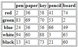
還是一樣先介紹一些相關的參數:
- Columns: 選擇要寫入的欄
df1.to_html('html100_1.html', columns=['key','pen','board'])
- col_space: 設定最小欄寬
df1.to_html('html100_1.html', col_space=100)
- header&index: 設定是否顯示header或index
df1.to_html('html100_1.html', index=False, header=False)
- float_format: 設定小數格式(建立df2,其中資料為float)
df2.to_html('html100_1.html', float_format="%.2f")
- justify: 設定欄標籤的邊靠位置,可選擇left、right、center、justify等
df1.to_html('html100_1.html', justify='left', col_space=100)
- bold_rows: 設定index是否為粗體,預設值為True
df1.to_html('html100_1.html', bold_rows=False)
- classes: 設定表格的class name以供CSS使用
df1.to_html('html100_1.html', classes="df1")
- max_rows& max_cols: 最多顯示行數與列數,預設值顯示全部
df1.to_html('html100_1.html', max_rows=3, max_cols=3)
- border: 設定表格邊線寬度
df1.to_html('html100_1.html', border=10)
- 如果想要在一頁寫入多個DataFrame,可以使用以下方式:
with open('html100_1.html', 'w') as f: f.write(df1.to_html() +"<br>" + df2.to_html())
現在可以在同一頁看到兩個表格。
dfList = pd.read_html('html100_1.html')之前提到可以在一頁中寫入超過一個表格,所以這裡特別命名為dfList,因為傳回值為一個list。若是要得到其中的DataFrame,毫無疑問要如下:
print(dfList[0])一樣再介紹一些相關屬性參數:
- Header: 設定header(最好是原本就沒有header時使用)
dfList = pd.read_html('html100_1.html', header=None)
- index_col: 設定index(最好是原本就沒有index時使用)
dfList = pd.read_html('html100_1.html', index_col=1)
- skiprows: 選擇不讀的row
dfList = pd.read_html('html100_1.html', skiprows=[1,3])
read_csv(filepath_or_buffer=”http://...html”)
,第一個參數是網路位址。前述做法都是跟檔案有關,以下介紹幾種其他的傳輸方式:
- to_dict(): 將熊貓資料轉換成dict
print(df1.to_dict()) print(df1.key.to_dict())
當然也可用於Series,例如使用df1.key.to_dict()(此方式與df1.key.tolist()傳回值不同)。其實此方法不只能將熊貓資料轉換成dict,設定參數也可以轉換成其他顯示形式,可用的選擇有dict(預設值)、 list、series、split、records、index等(除了預設值,Series並不支援其他參數)。print(df1.to_dict(orient='list')) print(df1.to_dict(orient='series')) print(df1.to_dict(orient='split')) print(df1.to_dict(orient='records')) print(df1.to_dict(orient='index'))
- to_frame(): 將Series轉換成DataFrame
print(df1.key.to_frame(name="newkey"))
- to_string(): 將熊貓資料轉換成字串
print(df1.to_string(header=False))
- to_json(): 將熊貓資料轉換成json
print(df1.to_json())
Json是網路傳輸常用之資料格式,原則上就是內容為dict的字串,你可以使用df1.to_dict()然後比較兩者看看。 - to_sql()&read_sql(): 將熊貓資料傳入資料庫與自資料庫讀出
在anaconda中我們可以使用以下方式使用簡易的資料庫:from sqlalchemy import create_engine
然後建立engine,便可以將資料傳入設立的資料庫內engine = create_engine('sqlite:///adb.db') df1.to_sql('dframe1', engine)
相當簡單,若是想要將其讀出,則使用read_sql()方法df1_sql = pd.read_sql('dframe1', engine) print(df1_sql)
- to_pickle()&read_pickle(): 將熊貓資料傳入資料庫與自資料庫讀出
pickle是Python內建的一種模組,也可以用來存儲資料(類似儲存到檔案),使用方式很簡單:import pickle df1.to_pickle('frame1.pkl')
這樣就能將資料儲存在pickle並給一個名稱,若要取得資料,只要給對應名稱即可:pickleframe1=pd.read_pickle('frame1.pkl')
你可以在對應資料夾中看到frame1.pkl這個檔案,有這個檔案可以讓我們以後都能讀取裡面的資料。
-
Talk100_1.py
- 使用to_html()將資料寫成html檔案
- 使用pd.read_html()來讀取html檔案中的table
- 使用to_dict()將熊貓資料寫成html檔案
- 使用to_frame()將Series轉換成DataFrame
- 使用to_string()將熊貓資料轉換成字串
- 使用to_json()將熊貓資料轉換成json
- 使用to_sql()&read_sql()將熊貓資料在資料庫存取
- 使用to_pickle()&read_pickle():將熊貓資料在硬碟存取
Recap
第一百零一話、熊貓之老生常談
之前花了好幾話的篇幅介紹熊貓的用法,現在用個例子來練習一下。熊貓的操作常常有一個動作可以對應好幾個指令的情況,這造成指令繁多的混亂情況,所以我們可以先熟悉每個動作的一個對應指令,用熟了之後,其他的類似指令要不要記得其實好像也無所謂對吧?不過反過來說記得越多指令可能越靈活。 以下例子關於兩組資料,資料儲存在兩個檔案內,分別為Senders.txt and Packages.txt,一個記載寄送人資料,一個記載包裹資料。因為內容有中文,所以先使用NotePad++開啟檔案,在右下角看編碼格式,若不是utf-8,到編碼>>轉換至utf-8格式,然後存檔。- 導入需要的模組
import numpy as np import pandas as pd
- 讀取檔案內容並存為DataFrame
senders = pd.read_csv("Senders.txt", index_col=0) packages = pd.read_csv("Packages.txt", index_col=0)
- 顯示前幾行觀察資料
print(senders.head()) print(packages.head())
- 觀察資料數量與型態 可以直接使用senders.shape與packages.shape來取得行數與列數,若僅想知道行數,也可以使用senders.shape[0]或是len(senders),抑或是印出senders.index也可看到行數。
print(senders.shape) print(packages.shape)
至於資料型態只要使用senders.dtypes即可。print(senders.dtypes)
也可以使用senders.info()來得到所有資訊。 - 在packages中有一欄為包裹內容,其中總共包含哪些內容?
print(packages.內容.unique())
- 各項包裹內容的總數為多少?又其中哪一項最少被寄送?
print(packages.內容.value_counts().head())
最少被寄送的品項:print(packages.內容.value_counts().tail(1))
- 描述資料的敘述統計
print(senders.describe()) print(packages.describe())
若是連非數字內容也要全部納入:print(packages.describe(include='all'))
- 自senders取得寄件人、包裹編號、與運費並依據寄件人及運費排序
shipper = senders[['寄件人','包裹編號','運費']] shipper = shipper.sort_values(['寄件人','運費']) print(shipper.head())
- 設定包裹編號為shipper的index並找出運費最高與最低的包裹編號
shipper.set_index('包裹編號', inplace=True) print(shipper.head(3))
- 根據index排序shipper
shipper.sort_index(inplace=True) print(shipper.head())
- 傳回運費超過190的包裹編號陣列
more190 = shipper[shipper.運費>190].包裹編號.tolist() print(shipper[shipper.運費>190].包裹編號.head())
- 列出運費最低及最高的5個包裹編號
print(shipper.運費.nsmallest()) print(shipper.運費.nlargest())
- 列出所有位於高雄的寄件人地址並取得符合此條件的運費總和
khaddress = senders.寄件人地址[senders.寄件人地址.str.find('高雄')!=-1]
或使用khaddress = senders.寄件人地址[senders.寄件人地址.str.contains('高雄')]
print(khaddress.head())
運費總和:print(senders.運費[senders.寄件人地址.str.find('高雄')!=-1].sum())
- 刪除khaddress中郵遞區號為830的資料
mask = khaddress[khaddress.str.find('830')!=-1].index khaddress = khaddress.drop(mask) print(khaddress[khaddress.str.find('830')!=-1].head())
- 重新設定khaddress的index
khaddress.reset_index(drop=True, inplace=True)
當然也能這麼做khaddress.index=range(len(khaddress))
- 找到Parker的托運資料之包裹編號與運費
print(senders.loc[senders.寄件人.isin(['Parker']),['寄件人','包裹編號','運費']])
或是這麼做:print(senders.query("寄件人=='Parker'")[['包裹編號','寄件人','運費']])
- 找到價值介於500~1000的包裹編號
print(packages.包裹編號[packages.價值.between(500, 1000)].head())
- 列出在2010年1月1日之前託運的包裹編號及日期
print(packages.loc[(cackages.運送日期-日期<"2010-01-01"),['包裹編號','運送日期']].head()]
- 列出在2010年1月1日之前託運且重量小於100的資料
print(packages[(packages.運送日期-日期<"2010-01-01")&(packages.重量<100)].head())
- 將兩個DataFrame根據包裹編號合併為一個
senderpack = senders.merge(packages, sort=True) print(senderpack.head(2))
- 在senderpack中增加一個欄位,內容是包裹運費與重量的比值
senderpack["運費重量比"] = senderpack.價值/senderpack.重量
- 將運費重量比四捨五入到小數後第二位
senderpack.運費重量比" = senderpack.運費重量比".apply(lambda x: np.round(x,2))
當然也可以直接使用senderpack.運費重量比"=senderpack.運費重量比".round(2)
- 根據寄件人分組,並計算各人的總運費
sendergroups = senderpack.groupby(by="寄件人") print(sendergroups.運費.sum().head(3))
- 列出平均運費最高的5人
print(sendergroups.運費.mean().nlargest(5))
- 根據寄件人與包裹內容分組,並列出某人寄送相同內容物品超過一次的組別
sc = senderpack.groupby(by=["寄件人","內容"]) for g, d in sc: if d.shape[0]>1: print(g,d.包裹編號)
Python亂談
matplotlib
第一百零二話、matplotlib
這裡開始介紹視覺化(visualization),主要就是介紹matplotlib這個模組,這是專門幫我們建立資料圖形顯示,可以完美搭配pandas使用,在使用時須先import matplotlib.pyplot這個模組。首先來看個簡單的例子:import numpy as np import pandas as pd import matplotlib.pyplot as plt np.random.seed(2019) list1 = [np.random.randint(1,100) for i in range(5)] ser1 = pd.Series(np.random.randint(1,100,5)) plt.plot(list1)使用plot()方法然後參數給定list、tuple或是series等類型資料,即可直接繪圖,如下:
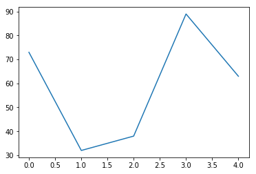
只要在圖上點右鍵即可複製圖片或存成圖檔。如果我們再加上
plt.plot(ser1)這一行,會不會繪製兩個圖?答案是不會,會將兩個折線圖都繪製在一起,如下:
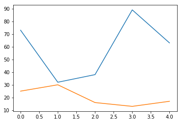
那麼如果是DataFrame(或是ndarray)的話,繪製出來的形式如下:
df1 = pd.DataFrame(np.random.randint(1,100,(5,5))) plt.plot(df1)
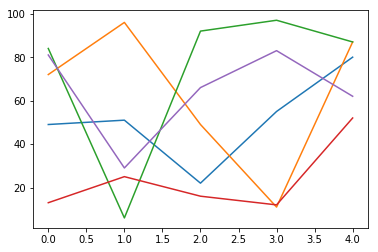
原則上就是每個column繪製一條折線圖。其實plot()方法的格式可為如下兩類:
plot([x], y, [fmt], data=None, **kwargs)
plot([x], y, [fmt], [x2], y2, [fmt2], ..., **kwargs) 前兩個參數是x與y,如果想要繪製超過兩組資料,則給兩組x與y。上述的例子都是使用資料作為y,x則為index編號,例如:
ser2 = pd.Series(np.random.randint(1,100,5), index=list("abcde")) plt.plot(ser2)
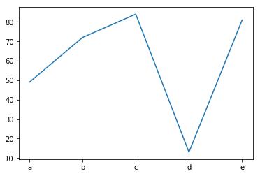
現在我們試著分別給x,y的值,例如:
x = np.random.randint(1,100,5) y = np.random.randint(1,100,5) plt.plot(x,y)
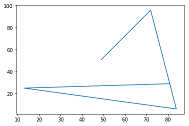
x = np.random.randint(1,100,5) y = np.random.randint(1,100,5) x2 = np.random.randint(1,100,5) y2 = np.random.randint(1,100,5) plt.plot(x,y,x2,y2)
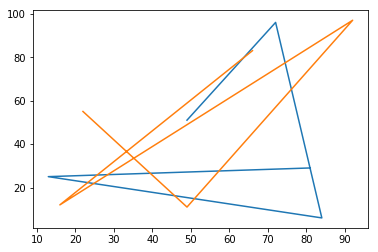
此例的x,y資料實在不適合繪製折線圖,應該繪製分布圖就好了,所以只要我們給一下format就可以:
plt.plot(x,y,"bo")

plt.plot(x,y,"bo",x2,y2,"r.")

非常的容易,有如桌頂拈柑。不過這個bo跟r.是甚麼東東?其實b就是blue,顯然就是red,而o代表的是較大的圓點,.表示的就是一個點 。以下列出可用的顏色跟圖形。
| b: blue | g: green | r: red |
| c: cyan | m: magenta | y: yellow |
| k: black | w: white | #rrggbb: 16進位法方式顯示 |
| '-' or 'solid | '--' or 'dashed' | '-.' or 'dashdot' | ':' or dotted | 'None' or '' or ' ' |
| '.' | ',' | 'o' | 'v' | '^' | '<' |
| '>' | '1' | '2' | '3' | '4' | '8' |
| 's' | 'p' | '*' | 'h' | 'H' | '+' |
| 'x' | 'X' | 'D' | 'd' | '|' | '_' |
| r"$\alpha$" | r"$\star$" | r"$\bigtriangleup$" |
| r"$+$" | r"$\sigma$" | r"$\spadesuit$" |
| r"$\imath$" | r"$\S$" | r"$\bigotimes$" |
| r"$\times$" | r"$\bigodot$" | r"$\bigoplus$" |
| r"$\Xi$" | r"$\Theta$" | r"$\oslash$" |
| r"$\beta$" | r"$\#$" | r"$\diamondsuit$" |
| r"$\ast$" | r"$\gamma$" | r"$\heartsuit$" |
| r"$\%$" | r"$\bullet$" | r"$\bigtriangledown$" |
| r"$\circ$" | r"$\$$" | r"$\bowtie$" |
| r"$\Phi$" | r"$\infty$" | r"$\clubsuit$" |
plt.plot(x,y,"c--")
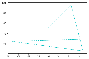
plt.plot(x,y,color="#ff00ff",marker=r"$\diamondsuit$",markersize=15)
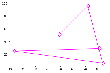
要注意的是如果使用參數來描述而不是使用類似”bo”,就不會出現散佈圖,而是出現點線混合的圖形。Plot()提供許多參數讓我們可以更豐富的圖形,以下為可用之參數:
- color: color = "#ff00ff"
- dashes: dashes(on, off)。e.g. dashes(5,5)
- dash_capstyle: 'butt','round','projecting'
- dash_joinstyle: 'miter', 'round','bevel'
- drawstyle: 'default', 'steps', 'steps-pre', 'steps-mid', 'steps-post'
- linestyle or ls: 'solid', 'dashed', 'dashdot', 'dotted', (offset, on-off-dash-seq) e.g. (10,(5,5,10,2)), '-', '--', '-.', ':', 'None','',' '
- fillstyle: fill the marker。'full', 'left', 'right', 'bottom', 'top', 'none'
- linewidth or lw: linewidth = 5
- marker: marker = r"$\beta$"
- alpha: alpha=0.5
- markeredgecolor or mec: mec = 'blue'
- markeredgewidth or mew: marker edge width,e.g. mew = 1.5
- markerfacecoloralt or mfcalt: mfcalt='pink'
- markerfacecolor or mfc: marker face color,e.g. mfc = "green"
- markersize or ms: ms = 10
- markevery: 每間隔幾個設置marker。'None', 'int', (a,b), list/array, float
- snap: 繪於格子點。snap=True(None)
- solid_capstyle: 'butt', 'round','projecting'
- solid_joinstyle: 'miter', 'round', 'bevel'
plt.plot(x,y,marker="o", color='blue', dash_capstyle="round", drawstyle='steps', fillstyle='left', ls=(10,(5,3,5,5)), mec = 'red', mew = 0.5, mfc = 'green', mfcalt = 'pink', ms = 20, markevery = (1,2))
-
Talk102_1.py
- 欲使用matplotlib繪製圖形需先import matplotlib.pyplot as plt
- 使用plot()方法來繪製圖形,可繪製多筆資料於一圖內
- 給定plot()方法參數來改變顯示內容
Recap
第一百零三話、再談matplotlib圖形顯示
上一話提到若是想要在一個圖中繪製多筆資料,可以直接加入x2,y2,再練習一下:import numpy as np import pandas as pd import matplotlib.pyplot as plt np.random.seed(103) x1 = np.arange(10,20) x2 = np.arange(1,11) y1 = pd.Series(np.random.randint(1,10,10)) y2 = pd.Series(np.random.randint(10,20,10)) plt.plot(x1,y1,'bo-',x2,y2,'r+--')
而我們也可以分別繪製兩組資料:
plt.plot(x1,y1,'bx-') plt.plot(x2,y2,color='red', marker = 'o', mfc="b", mec='b', ls=':')
如上一話所述,若是有label或是index的資料,可以直接當成x,資料當做y來繪製,例如:
dic1 = {'data_x1':x1, 'data_y1':y1} dic2 = {'data_x2':x2, 'data_y2':y2} plt.plot('data_x1','data_y1', 'gX-',data=dic1) plt.plot('data_x2','data_y2', data=dic2, marker = r"$\$$", ms=15, mfc='b',mec='b', ls='-.', color='r')
為何說pandas與matplotlib非常契合,因為pandas的資料可以直接呼叫plot()方法來繪製圖形,例如:
df1 = pd.DataFrame( np.random.randint(1,100,(10,2))) df1.plot()
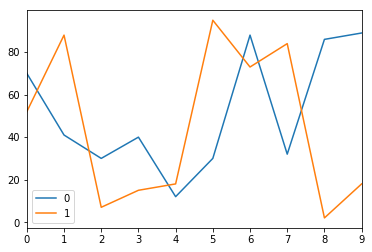
這個方式可以快速得到圖形,不過顯然使用plt.plot()的自由度較大 。除了繪製圖形,matplotlib還提供多樣的圖形修飾功能,這可以讓圖形更為詳盡及專業,首先看圖型大小與標題:
- plt.figure(figsize=(w,h)): 設定圖型大小,但要放在其他設定之前
figure(num=None, figsize=None, dpi=None, facecolor=None, edgecolor=None, frameon=True, FigureClass=, clear=False, **kwargs)
- plt.title(): 建立圖型的標題
plt.figure(figsize=(8,6), facecolor='#fa0af5') plt.title("Fig Title", fontsize=30, color="#58a7f9", fontname='Aharoni', pad=10, loc='center') plt.plot(x1,y1,'bx-', label="y1") plt.plot(x2,y2,color='red', marker = 'o', mfc="b",mec='b', ls=':', label='y2')
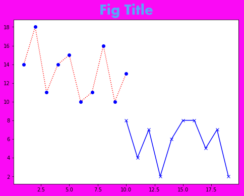
其中title可以使用fontsize, fontname,color, verticalalignment(top, center, baseline), horizontalalignment(left, center, right),pad,loc(left,center,right)來修飾
接下來看怎麼設定軸:
- plt.xlabel()與plt.ylabel(): 設定x,y軸的標題
- plt.axis(): 設定軸的數值範圍
- plt.tick_params(axis='both', **kwargs): 改變tick型態
- plt.minorticks_on()與plt.minorticks_off(): 開啟關閉minor ticks
plt.figure(figsize=(8,6), facecolor='#fa0af5') plt.title("Fig Title", fontsize=30, color="#58a7f9", fontname='Aharoni', pad=10, loc='center') plt.xlabel("x", color='white', fontsize=15, fontname='Broadway') plt.ylabel("y", color='white', fontsize=15, fontname='Broadway') plt.axis([0,20,0,20]) plt.tick_params(axis='y', labelcolor='silver',labelsize=15) plt.minorticks_on() plt.plot(x1,y1,'bx-', label="y1") plt.plot(x2,y2,color='red', marker = 'o', mfc="b",mec='b', ls=':', label='y2')
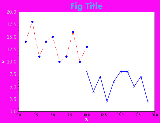
接下來如果我們想要加上格線、圖例與文字,使用:
- plt.grid(b=None, which='major', axis='both', **kwargs): 設定格線
- plt.legend(): 顯示圖例(位置可使用0到10,分別對應到best, upper right, upper left, lower left, lower right, right,center left, center right, lower center, upper center, center等位置)
- plt.text(x, y, s, fontdict=None, withdash=False, **kwargs): 可顯示文字於圖型(因為是文字性質,可使用文字的屬性參數,例如color)
plt.figure(figsize=(8,6), facecolor='#fa0af5') plt.title("Fig Title", fontsize=30, color="#58a7f9", fontname='Aharoni', pad=10, loc='center') plt.xlabel("x", color='white', fontsize=15, fontname='Broadway') plt.ylabel("y", color='white', fontsize=15, fontname='Broadway') plt.axis([0,20,0,20]) plt.tick_params(axis='y', labelcolor='silver',labelsize=15) plt.minorticks_on() plt.grid(True, color='lightgreen') plt.plot(x1,y1,'bx-', label="y1") plt.plot(x2,y2,color='red', marker = 'o', mfc="b",mec='b', ls=':', label='y2') for i in range(len(x1)): plt.text(x1[i], y1[i]+0.5, y1[i], color="orange") plt.text(x2[i], y2[i]+0.5, y2[i]) plt.legend(loc=0)
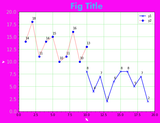
加入text時,會坐落在x,y位置,此處將y位置都+0.5,使其上移一些,避免與線條重疊過多。再加入legend之前,在plot()內加入label屬性參數來做為顯示,並記得將其放置於plot()之後。legend()也有其他參數,可以練習以下各寫法:
plt.legend(loc=0) plt.legend(loc=0, frameon=False) plt.legend(loc=0, frameon=False, ncol=2) plt.legend(loc=0, framealpha=0.7, shadow=True, borderpad=1)若是要讓圖形顯示特定的風格,可以導入matplotlib.style模組,然後使用use()方法,例如:
from matplotlib import style style.use("ggplot") plt.plot(x1,y1)

其中的ggplot為一種風格,若要查詢其他風格,可以使用style.available,如下:
plt.style.available請自行嘗試不同的繪圖風格。
-
Talk103_1.py
- 欲在一圖形中繪製多筆資料,可先行取出各筆資料的x,y,然後再各自繪入
- 使用plt.figure(figsize=(w,h))與plt.title()設定圖型大小與標題
- 使用plt.xlabel()、plt.ylabel()、plt.axis()、plt.tick_params()、plt.minorticks_on()、與plt.minorticks_off()等來設定軸
- 使用plt.grid()、plt.legend()、與plt.text()等來設定格線、圖例以及加入文字
- 導入matplotlib.style然後使用style.use()來改變繪圖風格
Recap
第一百零四話、matplotlib之多圖形顯示
之前提到在一個圖中顯示多筆資料,接下來談如何顯示多個子圖形的方式。主要的方法是subplot(),因為要將多個子圖形合為一個圖,所以先設計多個圖的資料如下:import numpy as np import pandas as pd import matplotlib.pyplot as plt np.random.seed(104) x1 = np.arange(10) y1 = np.random.randint(1,100,10) y2 = np.random.randint(1,100,10) y3 = np.random.randint(1,100,10) y4 = np.random.randint(1,100,10) y5 = np.random.randint(1,100,10)這些可以繪製5個不同的圖,接下來繪製兩個並列的圖:
plt.subplot(211) plt.plot(x1,y1,"bo") plt.subplot(212) plt.plot(x1,y2,"r--")
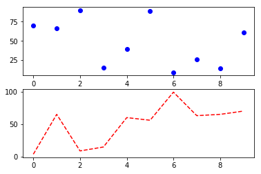
plt.subplot(1,2,1) plt.plot(x1,y1,"bo") plt.subplot(1,2,2) plt.plot(x1,y2,"r--")
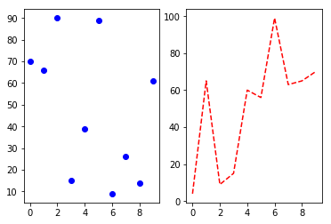
最讓人困惑的應該就是211、212這些數字了,211的意思是有2個row,1個column,其中的第一個圖。其餘依此類推。寫法也可以分開,變成2,1,1。原則上上述的圖形是被分為四小格的,所以如果改成這樣:
plt.subplot(2,2,1) plt.plot(x1,y1,"bo") plt.subplot(2,2,2) plt.plot(x1,y2,"r--")
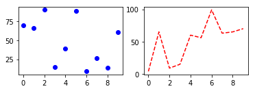
可以看出本來可以放四個圖,但是只放了兩個,所以小了點。接下來看若是一個圖會跨行或跨欄的做法,其實一開始的兩個圖就是跨行與跨欄的,做法如下:
plt.subplot(2,2,1) plt.plot(x1,y1,"bo") plt.subplot(2,2,2) plt.plot(x1,y2,"r--") plt.subplot(212) plt.plot(x1,y3,"g.-")
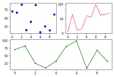
plt.subplot(2,2,1) plt.plot(x1,y1,"bo") plt.subplot(2,2,3) plt.plot(x1,y2,"r--") plt.subplot(122) plt.plot(x1,y3,"g.-")
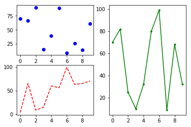
(221,222,212)是先將兩個較小的圖放在第一個row,然後跟之前一樣,第三個圖的212是放在有2-row,1-col的第二個圖。而(221,223,122)是先將兩個小圖放在2x2的1,3位置,然後第三個圖放置1-row,2-col的第二個位置。
上述的方法雖然似乎可以讓我們任意排放多個圖形,不過對於某些較為複雜的排列是有困難的,在這個情況下可以使用plt.GridSpec()方法,做法如下:
grid = plt.GridSpec(3,3,wspace=0.5,hspace=0.5, height_ratios=[1,1,3]) #right=2, top=2 to enlarge the figure >> height_ratios, width_ratios=[1,2,3] to change the size of each row or column plt.subplot(grid[0,0:3]) plt.plot(x1,y1,"bo") plt.subplot(grid[1,0:2]) plt.plot(x1,y2,"r--") plt.subplot(grid[2,0]) plt.plot(x1,y3,"g.-") plt.subplot(grid[2,1]) plt.plot(x1,y4,"cH") plt.subplot(grid[1:3,2]) plt.plot(x1,y5,"ms")
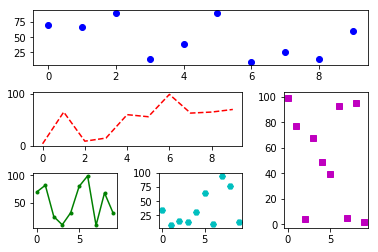
grid = plt.GridSpec(3,3,wspace=0.5,hspace=0.5) plt.subplot(grid[0,0:2]) plt.plot(x1,y1,"bo") plt.subplot(grid[0:2,2]) plt.plot(x1,y2,"r--") plt.subplot(grid[1:3,0:2]) plt.plot(x1,y3,"g.-") plt.subplot(grid[2,2]) plt.plot(x1,y4,"ms")
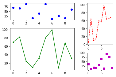
首先讓grid等於plt.GridSpec(),其中3,3表示是一個3x3的方格配置,wspace與hspace分別表示寬高方向圖與圖之間的間隔(將它們設為0看結果如何)。接下來就容易了,每一個subplot()內給的參數就是row與column的切片,row與column都是從0開始,例如grid[1:3,0:2]就是2到3行,1到2欄的空間。plt.GridSpec還有幾個參數可以應用,例如:
- 兩倍寬度:
grid = plt.GridSpec(3,3,wspace=0.5,hspace=0.5, right=2)
- 兩倍高度:
grid = plt.GridSpec(3,3,wspace=0.5,hspace=0.5, top=2)
- 三個欄寬的分配分別為1,2,3:
grid = plt.GridSpec(3,3,wspace=0.5,hspace=0.5, width_ratios=[1,2,3])
- 三個行高的分配為1,1,3:
grid = plt.GridSpec(3,3,wspace=0.5,hspace=0.5, height_ratios=[1,1,3])
fig, (ax1,ax2)=plt.subplots(1,2) ax1.plot(x1,y1,"bo") ax1.set_title('figure 1') ax2.plot(x1,y2,"r--") ax2.set_title('figure 2')
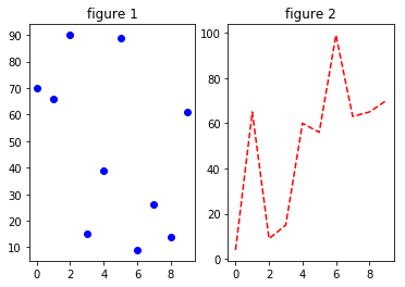
fig, (ax1,ax2)=plt.subplots(2,1) ax1.plot(x1,y1,"bo") ax1.set_title('figure 1') ax2.plot(x1,y2,"r--") ax2.set_title('figure 2')
Plt.subplots()會建立一個figure物件(fig)與一系列的子圖形(ax),參數(1,2)表示一個row,兩個column。直接使用ax.plot()即可繪圖。也可以使用以下方式來建立子圖。
fig, ax=plt.subplots(2,2) ax[0,0].plot(x1,y1,"bo") ax[0,1].plot(x1,y2,"r--") ax[1,0].plot(x1,y3,"gX") ax[1,1].plot(x1,y4,"m<")
如果要讓子圖的軸共用,可以使用sharex與sharey兩個參數屬性,可以給的值包括none、all、row、col、True、False等,例如:
fig, ax=plt.subplots(2,2, sharex='all', sharey='row') ax[0,0].plot(x1,y1,"bo") ax[0,1].plot(x1,y2,"r--") ax[1,0].plot(x1,y3,"gX") ax[1,1].plot(x1,y4,"m<")
跟上例相比,可以看到軸的數值現在是共用的。
-
Talk104_1.py
- 使用plt.subplot()方法來分隔圖形區域以做出多圖形
- 使用plt.GridSpec()方法來建立物件,此物件可以定義空間切片
- 使用plt.subplots()方法來建立格子圖以放置多圖形
Recap
第一百零五話、matplotlib之時間為軸
說到圖形的某一軸是時間,這馬上讓我們聯想到之前提過的pd.date_range()方法。想想好像沒甚麼困難的,畫個圖試試看:import numpy as np import pandas as pd import matplotlib.pyplot as plt np.random.seed(105) x1 = pd.date_range(start='2019-01-01', periods=20) y1 = np.random.randint(1,100,20) x2 = pd.date_range(start='2019-01-01', periods=31) y2 = np.random.randint(1,100,31) plt.subplot(2,1,1) plt.plot(x1,y1,'b-') plt.subplot(2,1,2) plt.plot(x2,y2,'ro')
原則上是沒問題,只是第一個圖的x軸顯示的文字都糾結在一起,第二個圖倒是沒問題。可見時間為軸的情況有可能讓顯示不清楚,若是想要讓顯示能夠清楚,可以嘗試使用如下方式:
import matplotlib.dates as mdates weeks = mdates.WeekdayLocator() days = mdates.DayLocator() timeFmt = mdates.DateFormatter('%y-%m-%d') fig,ax=plt.subplots() plt.plot(x1,y1,'b-') ax.xaxis.set_major_locator(weeks) ax.xaxis.set_major_formatter(timeFmt) ax.xaxis.set_minor_locator(days)
在這裡需先導入matplotlib.dates,然後使用其中的Locator方法,例如上例中的WeekdayLocator()與DayLocator()。而欲顯示的時間格是則使用mdates.DateFormatter()來定義。
當然也無法就此都能解決所有情況,例如:
x3 = pd.date_range(start='2019-01-01', periods=20, freq='M') y3 = np.random.randint(1,100,20) months = mdates.MonthLocator() weeks = mdates.WeekdayLocator() timeFmt = mdates.DateFormatter('%y-%m') fig,ax=plt.subplots() plt.plot(x3,y3,'rD') ax.xaxis.set_major_locator(months) ax.xaxis.set_major_formatter(timeFmt) ax.xaxis.set_minor_locator(weeks)
在這個情況下,只好稍作修正:
x3 = pd.date_range(start='2019-01-01', periods=20, freq='M') y3 = np.random.randint(1,100,20) months = mdates.MonthLocator() weeks = mdates.WeekdayLocator() timeFmt = mdates.DateFormatter('%m') fig,ax=plt.subplots() plt.plot(x3,y3,'rD') ax.xaxis.set_major_locator(months) ax.xaxis.set_major_formatter(timeFmt) ax.xaxis.set_minor_locator(weeks)
清楚了些,不過少了年的顯示。
-
Talk105_1.py
- 使用Locator來定義要顯示的時間,需先導入matplotlib.dates
- 使用DateFormatter()方法來定義顯示時間格式,並使用ax.xaxis.set_major_formatter()方法顯示
- 使用ax.xaxis.set_major_locator()與ax.xaxis.set_minor_locator()方法來定義主要跟次要的locator
Recap
第一百零六話、matplotlib之數學函數圖形
之前提到的都是一般資料的繪圖,那麼若是數學函數比如說sin()呢?其實很容易猜到,要繪製模擬連續函數,只要將點間間隔儘可能縮小看起來就接近了,當然間隔越小則資料量越大,例如:import numpy as np import pandas as pd import matplotlib.pyplot as plt x = np.arange(-2*np.pi, 2*np.pi, 0.1) y = np.sin(x) plt.text(-2.5, 0.75, 'y=sin(x)', fontsize=12, color='b', bbox={'facecolor':'y','alpha':0.5}) plt.plot(x,y)
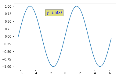
plt.text()是用來加上文字,其中bbox是關於文字框的屬性。
再來看下一個例子,此處要繪製心臟線,其公式為
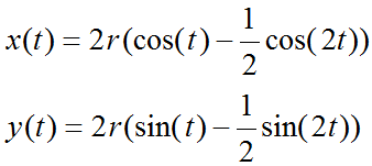
繪製方式如下:
plt.figure(figsize=[5,5]) t = np.arange(-5,5,0.01) r = 1 x = [2*r*(np.cos(i)-0.5*np.cos(2*i)) for i in t] y = [2*r*(np.sin(i)-0.5*np.sin(2*i)) for i in t] plt.plot(x,y)
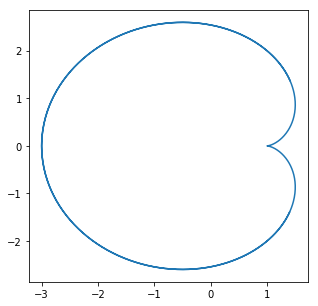
為了要讓圖形方正,所以設定figsize=[5,5],不然畫出來會看起來怪怪的。因為x與y都是t的函數,所以先設計t的內容。此處半徑r設為1。
下一步我們打算移動座標軸,讓其位於0的位置,如此看起來較像直角座標系。這一個圖有四個軸,分別為上下左右(top,bottom,left,right),做法是兩向各選擇一個留下,在此讓右及上隱藏,使用左與下。為了要控制軸,需要呼叫plt.gca(),此方法會傳回matplotlib.axes.Axes物件。取得物件後便可以使用spines[‘right’]來取得某一軸物件然後設定其屬性,如下:
ax = plt.gca() ax.spines['right'].set_visible(False) ax.spines['top'].set_color('none') ax.spines['bottom'].set_position(('axes', 0.5)) ax.spines['left'].set_position(('data', 0))
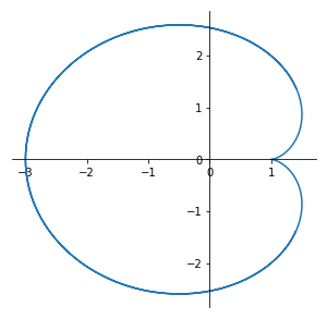
如上所述,ax為所取得的軸物件。使用set_visible(False)或set_color(‘none’)來讓其不可見。使用set_position()方法來改變軸的位置。
在set_position()方法中,輸入參數可以是data、axes及outward。data讓我們將軸放置在數值位置,axes讓我們移動軸到某比例位置,也就是可以輸入0~1之間的實數,例如輸入0.5會在正中間,如果大於1或小於0則會落於圖外。而outward則是讓座標軸坐落於圖外。
接下來可以加上數學式,我們可以這樣做
plt.text(-2.6,0.3,'x(t)=2r(cos(t)-(1/2)cos(2t))\ny(t)=2r(sin(t)-(1/2)sin(2t))', bbox={'facecolor':'y','alpha':0.5})

數學式看起來不是很正式,如果這樣呢?
plt.text(-2.7,0.5,r'$x(t)=2r(cos(t)-\frac{1}{2}cos(2t))$', bbox={'facecolor':'y','alpha':0.5}) plt.text(-2.7,-0.75,r'$y(t)=2r(sin(t)-\frac{1}{2}sin(2t))$', bbox={'facecolor':'y','alpha':0.5})
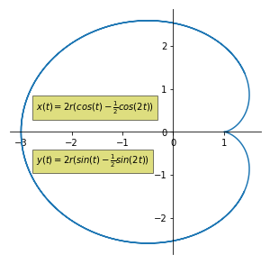
數學式看起來是好了點,不過無法一次顯示兩行。原來matplotlib提供數學表示法(TeX)讓我們可以顯示專業的數學寫法,以下為如何使用的介紹。
首先數學式的寫法模式是r’$symbol$’(之前在介紹點形式的時候也用過,見102話),其中r稱為raw string,這樣不會受到程式碼影響,例如上一個方程式若是加上r,那麼\n便會失效。而字串前後使用$標誌來確認此為數學方程式部分,數學式可以用在任何文字元件(例如plt.title())內。為了與其他文字做區別,使用\符號來表示特定符號。例如:
plt.title(r"$\alpha \gamma \omega$") |
 |
plt.title(r"$\# \$ \% \{ \}$") |
 |
- 字母與符號
plt.title(r"$\chi, \delta, \pi, \rho, \sigma$")
plt.title(r"$\Delta, \Omega, \Pi, \Psi, \Sigma, \Theta$")
plt.title(r"$\prod, \int, \oint, \iint, \iiint, \sum$")
- 三角函數與指對數
plt.title(r"$\sin, \cos, \tan, \cot, \sec, \csc$")

plt.title(r"$\arcsin, \arccos, \arctan$")

plt.title(r"$\log, \ln, \lg, \min, \max$")

- 上下標
plt.title(r"$x_1, x^2$")

plt.title(r"$\acute x, \bar x, \breve x, \ddot x, \dot x$")

plt.title(r"$\grave x, \hat x, \tilde x, \vec x, \overline{xyz}$")
plt.title(r"$\hat x, \widehat{xyz}, \widetilde{xyz}$")

- 分數或上下標同時(排列組合)
plt.title(r"$\frac{y}{x}, C\binom{5}{2}, C\stackrel{5}{2}$")

plt.title(r"$(\frac{y-\frac{y}{x}}{x})$")

plt.title(r"$\left(\frac{y-\frac{y}{x}}{x}\right)$")

- 根號
plt.title(r"$\sqrt{5}, \sqrt[3]{x}$")
- 極限、累加、微積分
plt.title(r"$\lim_{x\to 0}\frac{f(x)}{x}$")

plt.title(r"$\sum_{i=0}^\infty x_i$")

plt.title(r"$\int_{-\infty}^\infty xe^{-x^2} dx$")
plt.title(r"$\oint_{a(L_i)}^b q_0E^\bar w$")
plt.title(r"$\iiint xdV$")

- 字型(mathrm, mathit, mathtt,mathcal,mathbb, mathfrak,mathsf)
plt.title(r"$\mathcal{xyz},\mathfrak{xyz},\mathbb{xyz}}$")
x = np.arange(-5*np.pi,5*np.pi,0.01) y = (1-np.cos(x))/x plt.plot(x,y) plt.text(-13, 0.3, r'$y=\frac{1-\cos (x)}{x}$', fontsize=16, color='#ff00ff', bbox = {'facecolor':'#0af0bc', 'alpha':0.5}) plt.xticks([-5*np.pi, -4*np.pi, -3*np.pi, -2*np.pi, -np.pi, 0, np.pi, 2*np.pi, 3*np.pi, 4*np.pi, 5*np.pi], [r'$-5\pi$',r'$-4\pi$',r'$-3\pi$', r'$-2\pi$',r'$-\pi$',0, r'$\pi$', r'$2\pi$',r'$3\pi$',r'$4\pi$',r'$5\pi$'])
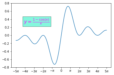
此處的求解函數與函數曲線皆以如前所述的方法繪製,我們額外使用plt.xticks()方法來改變x座標上的顯示(顯然可以使用plt.yticks()來改變y座標的顯示),方法中包含兩個參數,第一個稱為locs,代表坐標軸位置,第二個參數稱為labels,代表對應位置的顯示符號。
接下來可以一樣移動座標軸,如下:
ax=plt.gca() ax.spines['right'].set_visible(False) ax.spines['top'].set_visible(False) ax.spines['left'].set_position(('data',0)) ax.spines['bottom'].set_position(('data',0))
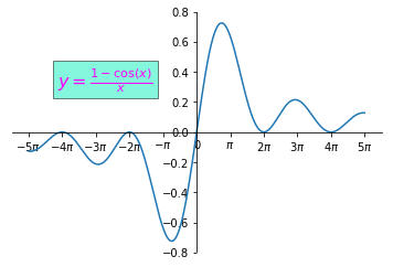
做法如前,不再贅述。最後再加上一個某一點的註解說明,此處取x趨近於0,只要加上以下的程式碼:
plt.annotate(r'$\lim_{x\to 2\pi}\frac{1-\cos (x)}{x}=0$', xy=[0, 0], xycoords='data', xytext=[3,-0.5], fontsize=16, arrowprops=dict(arrowstyle="->", connectionstyle="bar, armA=20,armB=13, fraction=0.1"))
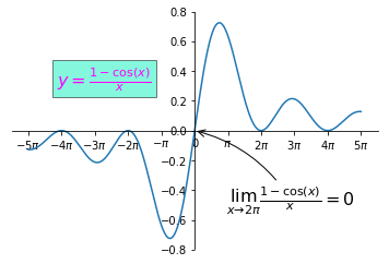
使用plt.annotate()方法,其中第一個參數是要顯示個數學公式,根據之前的做法可以輕易地完成。第二個參數xy表示要註解的座標點。第三個參數xycoords表示顯示xy的座標系統,這裡給值data(預設值),表示使用的數值所形成的座標系統。而xytext參數指的是註解(左上角)顯示的位置,fontsize是文字大小,應該不需說明。最後的arrowprops是用來描述指向該點的線段,須為一個dict。若是使用arrowstyle來描述箭頭形式,可以有以下選擇: -、->、-[、|-|、-|>、<-、<->、<|-、<|-|>、fancy、simple、wedge。
至於connectionstyle是描述連結的線段,除了arc3之外還可以有如下選擇(小括號內為預設值):
- angle, angleA=120(90), angleB=30(0)
- angle3, angleA=120(90), angleB=30(0)
- arc, angleA=0, angleB=0
- bar, armA=20(0),armB=15(0), fraction=0.1(0.3)
-
Talk106_1.py
- 建立小間距數列來繪製連續數學函數
- 使用plt.gca()方法來取得axes物件,然後使用spines[]來得到單獨軸,並指派屬性數值
- 使用set_position((‘data’,0))來將軸移至原點位置
- 使用plt.text()方法來配置文字或方程式
- 使用matplotlib內建的數學式建立方式顯示數學式
- 使用plt.xticks()或plt.yticks()方法來改變座標軸上的顯示值
- 使用plt.annotate()方法來建立註解
Recap
第一百零七話、matplotlib之顯示圖片
為了要讀取圖片,在此要額外導入from scipy.misc import imread
模組(或是導入import matplotlib.image as mpimg
然後使用mpimg.imread()),之後使用plt.imshow()方法來顯示圖片。先看一個例子:import numpy as np import matplotlib.pyplot as plt from scipy.misc import imread img1 = imread('./pics/pic1.jpg') plt.axis('off') plt.imshow(img1)
相當容易就可達成,不過旁邊的座標似乎是多餘的,此時只要加上
plt.axis('off')即可去除座標軸。我們可以改變圖形的色調,先將圖片的數值乘以[R,G,B]三色調,然後使用np.uint8()將其改為uint8格式。例如:
import matplotlib.image as mpimg img1 = mpimg.imread('./pics/pic1.jpg') img1_tinted=img1*[0.7, 0.7, 0.5] plt.axis('off') plt.imshow(np.uint8(img1_tinted))

可以藉由調整RGB(紅綠藍)三色的比例來調整色調。
若是印出img1數值來觀察,可看出它原則上是一個多維ndarray,每一個內層list表示一個pixel,三個數字表示RGB的值。也可以用如下方式(pseudocolor schemes)來修正顏色,這次應用於黑白照片:
import matplotlib.image as mpimg img4 = mpimg.imread('pics/pic4.jpg') plt.figure(figsize=[10,10]) plt.subplot(1,2,1) plt.imshow(img4) plt.subplot(122) img4_tinted=img4[:, :, 0] plt.axis('off') plt.imshow(img4_tinted)

上例右圖的色調其實是由cmap這個參數控制,預設值為viridis,我們可以藉由修改此參數的設定來改變色調,而cmap有許多可使用的值供選擇,計有如下,
Accent, Accent_r, Blues, Blues_r, BrBG, BrBG_r, BuGn, BuGn_r, BuPu, BuPu_r, CMRmap, CMRmap_r, Dark2, Dark2_r, GnBu, GnBu_r, Greens, Greens_r, Greys, Greys_r, OrRd, OrRd_r, Oranges, Oranges_r, PRGn, PRGn_r, Paired, Paired_r, Pastel1, Pastel1_r, Pastel2, Pastel2_r, PiYG, PiYG_r, PuBu, PuBuGn, PuBuGn_r, PuBu_r, PuOr, PuOr_r, PuRd, PuRd_r, Purples, Purples_r, RdBu, RdBu_r, RdGy, RdGy_r, RdPu, RdPu_r, RdYlBu, RdYlBu_r, RdYlGn, RdYlGn_r, Reds, Reds_r, Set1, Set1_r, Set2, Set2_r, Set3, Set3_r, Spectral, Spectral_r, Wistia, Wistia_r, YlGn, YlGnBu, YlGnBu_r, YlGn_r, YlOrBr, YlOrBr_r, YlOrRd, YlOrRd_r, afmhot, afmhot_r, autumn, autumn_r, binary, binary_r, bone, bone_r, brg, brg_r, bwr, bwr_r, cividis, cividis_r, cool, cool_r, coolwarm, coolwarm_r, copper, copper_r, cubehelix, cubehelix_r, flag, flag_r, gist_earth, gist_earth_r, gist_gray, gist_gray_r, gist_heat, gist_heat_r, gist_ncar, gist_ncar_r, gist_rainbow, gist_rainbow_r, gist_stern, gist_stern_r, gist_yarg, gist_yarg_r, gnuplot, gnuplot2, gnuplot2_r, gnuplot_r, gray, gray_r, hot, hot_r, hsv, hsv_r, inferno, inferno_r, jet, jet_r, magma, magma_r, nipy_spectral, nipy_spectral_r, ocean, ocean_r, pink, pink_r, plasma, plasma_r, prism, prism_r, rainbow, rainbow_r, seismic, seismic_r, spring, spring_r, summer, summer_r, tab10, tab10_r, tab20, tab20_r, tab20b, tab20b_r, tab20c, tab20c_r, terrain, terrain_r, viridis, viridis_r, winter, winter_r
有點多,隨便試兩個看看:import matplotlib.image as mpimg img4 = mpimg.imread('pics/pic4.jpg') img4_tinted=img4[:, :, 0] plt.figure(figsize=[10,10]) plt.axis('off') plt.subplot(1,2,1) plt.imshow(img4_tinted,cmap='Oranges') plt.subplot(122) plt.imshow(img4_tinted,cmap='coolwarm')

現在順便複習使用GridSpec()來繪製子圖如下:
from scipy.misc import imread img1 = imread('pics/pic1.jpg') img2 = imread('pics/pic2.jpg') img3 = imread('pics/pic3.jpg') img4 = imread('pics/pic4.jpg') img4_tinted=img4[:, :, 0] plt.figure(figsize=[10,10]) grid=plt.GridSpec(2,2,wspace=0.1) plt.subplot(grid[0,0]) plt.axis('off') plt.imshow(img1) plt.subplot(grid[0,1]) plt.axis('off') plt.imshow(img2) plt.subplot(grid[1,0]) plt.axis('off') plt.imshow(img3) plt.subplot(grid[1,1]) plt.axis('off') plt.imshow(img4_tinted,cmap='hot')

-
Talk107_1.py
pic1.jpg
pic2.jpg
pic3.jpg
pic4.jpg
- 需額外導入from scipy.misc import imread模組或import matplotlib.image as mpimg
- 使用imread()方法讀取圖片,並使用plt.imshow()方法顯示圖片
- 將圖片數值乘以特定比例,可調整圖片色調,或使用pseudocolor schemes方法,藉由修改cmap參數來調整色調
Recap
第一百零八話、matplotlib之散佈圖
其實我們之前就提過可以使用plt.plot()方法來建立散佈圖了,只是好像不太正統,因為若是給參數就會變成點加線混合的圖,例如:import numpy as np import pandas as pd import matplotlib.pyplot as plt np.random.seed(108) x = np.random.randint(1,100,10) y = np.random.randint(1,100,10) plt.plot(x,y,marker='o',markersize=10, color='red',mfc='blue',mec='blue')

雖然可以使用例如plt.plot(x,y,’ro’)來繪製散佈圖,卻缺少了彈性。所以正統的散佈圖,應該使用scatter()方法,例如:
plt.scatter(x,y,marker='o',s=50, c='red',alpha='0.8', linewidths=1, edgecolors='blue')
注意此處與plot()不同,使用s表示大小,c表示顏色,而alpha是不透光度,linewidths表示點外圍線段寬度,edgecolors表示其顏色。顏色除了使用十六進位,也可以使用0~1表示比例,例如:
plt.scatter(x,y,marker=r'$\clubsuit$', s=200, alpha='0.8', c=[[0.9,0.1,0.5]], linewidths=0.5, edgecolors='blue') for i in range(len(x)): plt.text(x[i]+1,y[i]+0.2,i)
若資料是儲存成DataFrame,除了使用plt.scatter(),也可以直接使用plot()方法,例如:
df1 = pd.DataFrame( np.random.randint(1,100,(10,2)), columns=['A','B']) df1.plot(x='A',y='B',kind="scatter", c="#f00ff0")
也可以寫成
df1.plot.scatter(x='A',y='B',c="#f00ff0")效果是一樣的。記得x與y分別為某一column。
-
Talk108_1.py
- 使用plt.scatter()方法來繪製散佈圖
- 參數s代表點大小,c代表顏色
- DataFrame可以直接使用plot()方法繪製
Recap
第一百零九話、matplotlib之長條圖
有折線圖與散布圖,當然有長條圖。使用的方法為bar(),例如:import numpy as np import pandas as pd import matplotlib.pyplot as plt np.random.seed(109) x = pd.Series(list("abcdefghij")) y = np.random.randint(1,100,10) plt.bar(x,y)
用法都類似,給了x與y的list-like結構的數值,即可輕鬆的繪製。當然我們可以修改一些參數來讓圖形更為豐富多變。將上例的plt.bar()換成如下:
plt.bar(x,y,width=0.5,bottom=10,align='center', color='red',linewidth=2.5, edgecolor='green', tick_label=np.arange(1,11))
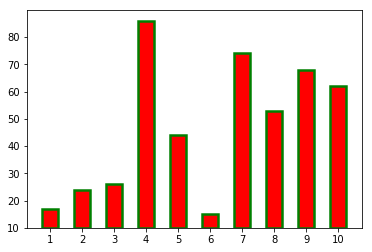
其中width是指長條的寬度,預設值為0.8。bottom指的是y的最小數值,預設值為0。Align是長條對應x-tick的位置,可以選擇center或edge。
使用edge的話tick會對應到長條的左邊,若是要對應到右邊,則把width的值變成負的即可。Linewidth與edgecolor分別對應長條的邊框寬度與顏色。而tick_label顯然是修改x軸tick的顯示。也可以使用
plt.xticks(x,np.arange(1,11))來修改。再看另一個顯示的例子:
np.random.seed(109109) y1 = np.random.randint(10,10000,10) plt.bar(x,y1,width=-0.5,bottom=10,align='edge', color='red',linewidth=2.5, edgecolor='blue', log=True, fill=False, alpha=0.5, hatch="///") plt.xlabel('x', color='olive', fontsize=15) plt.ylabel('y', color='olive', fontsize=15) plt.tick_params(axis='y',labelcolor='red') plt.title('Bar Chart', fontsize=30, color='tomato',pad=10) plt.grid(True)
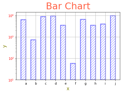
這次又加了幾個新參數並將之前提過的圖形修飾加上去。新參數的部分首先看log=True,這表示y軸使用對數形式。而alpha是不透光度,這是我們已知的。再來看fill=False,這表示不使用顏色填滿,所以color=’red’變得無效,而我們使用hatch參數來使用圖案填滿,hatch可以選擇的種類有/、\\、 |、-、+、x、o、O、.、*。其中只有\\需要雙數,因為\是特殊符號,使用兩個來表示一個。我們若想讓線條或點點密度高,就多寫幾個,例如上例中的///。
有直的長條圖,顯然也有橫的長條圖。因為參數幾乎都一樣,所以事情就容易多了,把bar()改為barh()、width改為height、bottom改為left,如下:
plt.barh(x,y,height=0.5,left=10,align='center', color='red',linewidth=2.5, edgecolor='blue', fill=False, alpha=0.5, hatch="|||") plt.xlabel('y', color='olive', fontsize=15) plt.ylabel('x', color='olive', fontsize=15) plt.tick_params(axis='y',labelcolor='red') plt.title('Bar Chart', fontsize=30, color='tomato',pad=10) plt.grid(True)
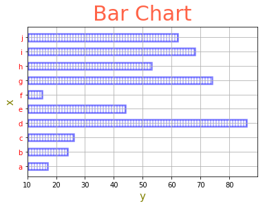
參數原則上都跟直長條圖相同,主要要記得修改成height與left。在長條圖的表示中,有時候我們會想表示錯誤容許值,這個時候做法如下:
err = [2 for i in range(10)] plt.bar(x,y,width=0.5,bottom=10,align='center', linewidth=2.5, edgecolor='blue', fill=False, alpha=0.5, hatch="///", yerr=err, error_kw={'ecolor':'brown','capsize':6}) plt.xlabel('x', color='olive', fontsize=15) plt.ylabel('y', color='olive', fontsize=15) plt.tick_params(axis='y',labelcolor='red') plt.title('Bar Chart', fontsize=30, color='tomato',pad=10) plt.grid(True)
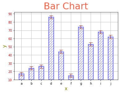
若是橫向長條圖,要使用xerr參數。而error_kw是一個dict,可以用來修飾其顏色或是橫蓋的長度。
另一個情況是若是我們想要顯示一個x值對應到多個y值的長條圖,那麼做法如下:
x = np.arange(1,11) y1 = np.random.randint(1,100,10) y2 = np.random.randint(1,100,10) y3 = np.random.randint(1,100,10) err = [2 for i in range(10)] gap=0.3 plt.barh(x,y1,height=gap,left=10,align='center', color='green', xerr=err, label="data 1", error_kw={'ecolor':'b','capsize':3}) plt.barh(x+gap,y2,height=gap,left=10,align='center', fill=False, alpha=0.5, hatch="|||", label="data 2", xerr=err, error_kw={'ecolor':'b','capsize':3}) plt.barh(x+2*gap,y3,height=gap,left=10,align='center', color='red', xerr=err, label="data 3", error_kw={'ecolor':'b','capsize':3}) plt.yticks(x+gap, x) plt.xlabel('y', color='olive', fontsize=15) plt.ylabel('x', color='olive', fontsize=15) plt.tick_params(axis='y',labelcolor='red') plt.title('Bar Chart', fontsize=30, color='tomato',pad=10) plt.grid(True) plt.legend()
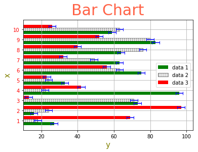
此處使用橫向長條圖做為例子。要顯示三筆資料,直接使用plt.barh()繪製三次即可。因為怕太紊亂,所以省略了長條的邊框,並將height縮小至0.3。且capsize也縮小至3。要注意的是此處將x修正為數字,因為每繪製一個長條圖,都平移一個gap的寬度,這樣圖才不會疊在一起,所以要記得讓x+gap與x+2*gap。為了讓y軸的tick對應到三個長條的正中間,所以使用plt.yticks(x+gap,x)指令來移動tick。直向長條圖的做法類似。
-
Talk109_1.py
- 使用plt.bar()方法來繪製長條圖,並利用width、bottom、align、color、linewidth、edgecolor、tick_label、log、fill、alpha、hatch等參數來修飾
- 使用plt.barh()方法來繪製橫向長條圖
- 使用yerr或xerr參數來表示容許錯誤,並使用error_kw來修飾
- 欲繪製多重長條圖,要記得調整每個長條圖的位置使其正常顯示
Recap
第一百一十話、再談matplotlib之長條圖
除了前一話的直橫長條圖,matplotlib也可以繪製累加長條圖,舉例如下:import numpy as np import pandas as pd import matplotlib.pyplot as plt np.random.seed(110) x = pd.Series(list("abcde")) y1 = np.random.randint(1,10,5) y2 = np.random.randint(1,10,5) y3 = np.random.randint(1,10,5) plt.title("Stacked Bar Chart", fontsize=16, color='b') plt.bar(x,y1,color='b',label='Data 1') plt.bar(x,y2,color='g',label='Data 2', bottom=y1) plt.bar(x,y3,color='r',label='Data 3', bottom=y1+y2) plt.legend()
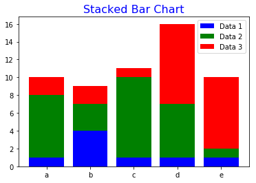
使用的指令與直條圖相同,都是bar(),主要需要修改bottom參數,讓後面的疊加到之前的數值之上,所以讓bottom=y1與bottom=y1+y2,其餘的皆相同。若是橫向的做法類似:
plt.title("Horizontal Stacked Bar Chart", fontsize=16, color='b') plt.barh(x,y1,color='b',label='Data 1', hatch="//") plt.barh(x,y2,color='g',label='Data 2', left=y1, hatch="++") plt.barh(x,y3,color='r',label='Data 3', left=y1+y2, hatch="oo") plt.legend()
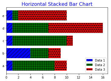
做法類似,除了須使用barh()方法之外,還要記得將bottom改為left參數即可,長條圖都可以使用hatch來增加變化。除了累加長條圖之外,還可以繪製雙向長條圖,例如:
plt.title("Bi-Direction Bar Chart", fontsize=16, color='b') plt.ylim(-10,10) plt.bar(x,y1,color='b',width=0.5, label='Data 1') plt.bar(x,-y2,color='g',width=0.5, label='Data 2') for i in range(5): plt.text(i, y1[i]+0.2, y1[i], color='r', ha="center", va="bottom") plt.text(i, -y2[i]-1, y2[i], color='r', ha="center", va="bottom") plt.grid(True) plt.legend()
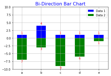
可以使用plt.ylim()控制y軸的顯示範圍。記得要將另一項的資料數值乘以負號,如上之-y2[i]。此外,使用plt.text()寫上長條的數值,為了對齊文字,加上ha(horizontal alignment)與va(vertical alignment)兩參數。若是橫向的做法類似:
plt.title("Bi-Direction Bar Chart", fontsize=16, color='b') plt.xlim(-10,10) plt.barh(x,y1,color='b', height=0.5, label='Data 1') plt.barh(x,-y2,color='g', height=0.5, label='Data 2') for i in range(5): plt.text(y1[i], i, y1[i], color='r', ha="left", va="center") plt.text(-y2[i]-0.5, i, y2[i], color='r', ha="left", va="center") plt.grid(True) plt.legend()
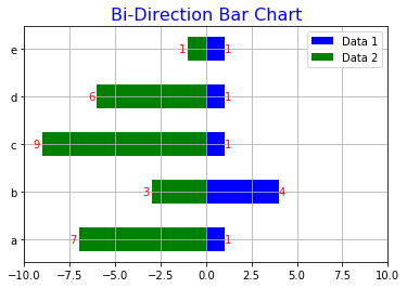
一樣要記得使用height代替width。使用plt.text()時也要記得x與y方向不同,並設定ha與va兩參數。
除了之前介紹的長條圖之外,還可以使用hist()方法繪製統計長條圖,做法如下:
plt.title("Histogram", fontsize=16, color='b') x = np.random.randn(1000) plt.hist(x, bins='auto', rwidth=0.7) plt.grid(True) plt.legend()
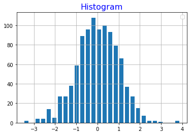
np.random.randn(1000)會產生1000個符合常態分配的數值。使用plt.hist()方法便可以繪製統計分配圖,其中bins是長條個數,可以使用auto或是給整數。rwidth表示每一個bar的寬度。長條圖也一樣可以使用DataFrame的plot()方法直接繪出,例如:
df1 = pd.DataFrame(np.random.randint(1,100,(10,3))) df1.plot(x=df1.index, y=[0,1,2], kind='bar', grid=True, title="DF Chart", rot=-30, ylim=[0,120])
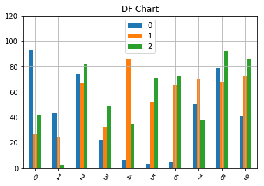
若是資料儲存為DataFrame格式,那麼使用plot()來繪製圖形不失為一個好用簡易的方法。其中的rot指的是x軸文字的旋轉角度。
使用df.plot()還可以有一些有趣的變化,例如:
df1 = pd.DataFrame(np.random.randint(1,100,(10,3))) df1.plot(x=df1.index, y=[0,1,2], kind='barh', grid=True, title="DF Chart", rot=-30, ylim=[0,120], cmap='tab20b_r', table=True)
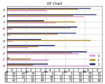
使用colormap(cmap)可以建立不同風格的顏色,參數同107話的cmap。Table這個參數可以幫我們將數值列出在一個表格內。其他型態的長條圖也可藉由修改kind參數來繪製。
-
Talk110_1.py
- 使用plt.bar()方法並控制bottom參數來形成累加長條圖,若是橫向則使用plt.barh()方法並控制left參數來繪製橫向累加長條圖
- 控制y數值的正負來繪製雙向長條圖並在使用plt.text()方法時設定ha與va參數來對齊文字
- 使用plt.hist()繪製統計長條圖
- 使用DataFrame的plot()方法直接繪出長條圖
Recap
第一百一十一話、matplotlib之圓型的圖
圓型的圖是統稱顯示成圓型的圖。其中圓餅圖就是pie chart,不多說,看以下例子:import numpy as np import pandas as pd import matplotlib.pyplot as plt np.random.seed(111) x = pd.Series(list("ABCDE")) y = np.random.randint(1,10,5) plt.pie(y, labels=x)

使用pie()方法便可繪製,不過要注意的是第一個參數是y值,而第二個參數為labels,是x的值,切勿搞混。
雖說是圓餅圖,不過看起來並不很圓,我們可以透過修正參數值來改善,如下:
plt.title('Pie Chart', fontsize=16, color='b') plt.pie(y, labels=x, explode=[0.15,0,0,0,0], startangle=0, shadow=True, autopct='%.2f%%', rotatelabels=True, counterclock=False, labeldistance=1.1) plt.axis('square')
看起來大不同。要變成正圓主要是因為plt.axis()方法改變了顯示軸,除了scaled之外,還可以選擇tight, on, off, image, equal, auto, normal, square等參數,請自行修改試驗。
explode參數決定其中某塊的位置,上例中是第一個,移動距離為0.15。而startangle則是第一個數值的起始角度,此處為0,所以A的起始角度為0。Autopct很明顯就是顯示數值的格式,圓餅圖原則上都是顯示比例。rotatelabels決定label是否旋轉,conterclock決定是否逆時針方向,而labeldistance表示繪製label的半徑。
接著來看雷達圖,做法如下:
def randomColor(): c = [np.random.choice(list("0123456789abcdef")) for i in range(6)] return '#'+''.join(c) n = 5 theta = np.arange(0,2*np.pi,2*np.pi/n) radii = np.random.randint(1,10,n) plt.axes([0,0,1,1],polar=True) plt.bar(theta,radii,width=(2*np.pi/n), bottom=0, color=[randomColor() for i in range(n)])

為了讓每個bar的顏色都不同,所以設計randomColor()函數來隨機產生顏色。為了在圓型上展現,將原來的x改為角度的theta。
使用plt.axes()來修正軸線,第一個參數是圖形大小,list內為左上角及右下角座標,最主要要記得設定polar=True。接下來就只是把長條圖畫上去,設定寬度讓360都被填滿,bottom=0表示底部在圓心。長條圖看起來比較好看,也可以使用散佈圖,如下:
plt.scatter(theta,radii, s=50, color=[randomColor() for i in range(n)])
看來使用長條圖應該是比較容易看出數值的。此外,在subplot()中有一個參數projection,設定其值為polar可以讓我們繪製極座標的圖形,這個方式可以繪製數學圖形,例如:
t = np.arange(0, 2, 0.01) r=5 ro = r*(np.sin(t)-np.cos(t)) ax = plt.subplot(111, projection='polar') ax.set_rticks([0.5,1,1.5,2]) ax.set_rlabel_position(90) ax.plot(ro, t, color='b')
因為我們只有要繪製一個圖,所以在subplot()內給定111,因為要使用極座標,所以設定參數projection為polar。
ax.set_rticks()可以讓我們設定要顯示的tick內容,在此可以讓圖形中的tick label顯示較少,免得看起來很紊亂。再者,使用ax.set_rlabel_position()可以控制label的位置,90表示90度的位置,這樣可以盡量避免label跟圖形的重疊。
其實繪製極座標圖形也可以直接使用plt.polar()方法,來試試看之前提過的心臟線:
t = np.arange(0, 2*np.pi, 0.01) r=1 ro = 2*r*(1-np.cos(t)) plt.polar(t,ro,color='b')

非常容易,跟數學課本上面教的一樣。不過軸的tick顯示倒是混在一起,此時若想調整,可以像前例一般利用subplot()取得axis,然後再做控制。
t = np.arange(0, 2*np.pi, 0.01) r=1 ro = 2*r*(1-np.cos(t)) ax = plt.subplot(111, polar=True) ax.set_rticks([1,2,3,4]) ax.set_rlabel_position(0) plt.polar(t,ro,color='b')
此處在subplot()內設定polar=True,原則上與前例中設定參數projection為polar效果相同。
現在練習繪製公式為 的rose curve,做法如下:
theta = np.arange(0, 2*np.pi, 0.01) r=3 k=9 ro = r*(np.cos(k*theta)) ax = plt.subplot(111, polar=True) ax.set_rlim(0,4) ax.set_xticks(np.arange(0, 2*np.pi, np.pi/6)) ax.set_rticks(np.linspace(0,3,4)) ax.set_rlabel_position(15) plt.polar(theta, ro, color='b', label='rose') plt.legend(loc=0)
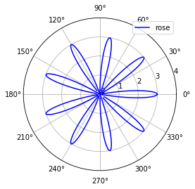
其中額外設定ax.set_ylim(0,4)(或set_rlim())來讓y軸的範圍大一些,主要是希望legend不要壓到圖上。並且多設定一個ax.set_xticks()來改變角度顯示的內容。若是要同時顯示兩個,只要再多繪製一個圖即可,做法如下:
theta = np.arange(0, 2*np.pi, 0.01) r=3 k=16 ro = r*(np.cos(k*theta)) ro2 = r*(np.sin(k*theta)) ax = plt.subplot(111, polar=True) ax.set_rlim(-5,5) ax.set_xticks(np.arange(0, 2*np.pi, np.pi/6)) ax.set_rticks(np.linspace(-5,4,10)) ax.set_rlabel_position(15) plt.polar(theta, ro, color='b', label='rose') plt.polar(theta, ro2, color='r', label='rose') plt.legend(loc=0)
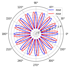
做了點參數修改,讓繪製的圖形有點變化。一樣的做法再舉個例子:
t = np.arange(0, 15*np.pi, 0.01) r=3 ro = r*(np.cos(t*np.pi))*(np.cos(t)) ro2 = r*(np.cos(t*np.pi))*(np.sin(t)) ax = plt.subplot(111, polar=True) ax.set_ylim(0,4) ax.set_xticks(np.arange(0, 2*np.pi, np.pi/6)) ax.set_rticks(np.linspace(0,3,4)) ax.set_rlabel_position(15) plt.polar(t,ro,color='b',label='rose') plt.polar(t,ro2,color='r',label='rose') plt.legend(loc=0)

-
Talk111_1.py
- 使用plt.pie()方法來繪製圓餅圖,並使用plt.axis()來改變軸型態
- 設定plt.axes(polar=True)來建立雷達圖
- 使用subplot()並設定projection='polar'來繪製極座標圖形,使用set_ylim()、set_xticks()、set_rticks()、set_rlabel_position()等方法來修飾圖形
- 使用plt.polar()方法直接繪製極座標圖
Recap
第一百一十二話、matplotlib之其他圖形
Matplotlib還可以繪製很多不同的圖,這裡來談一些沒有被歸類的圖形,第一個是等高線圖,舉例說明:import numpy as np import pandas as pd import matplotlib.pyplot as plt np.random.seed(112) x = np.arange(-3,3,0.01) y = np.arange(-3,3,0.01) m,n = np.meshgrid(x,y) def z(a,b): u=(1-a**5+b**5) v=np.exp(-a**2-b**2) return u*v ax = plt.subplot(111) plt.contour(m,n,z(m,n), 8)
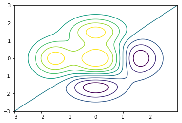
等高線圖應為三維,所以需要有個z方向的值,在此先使用np.meshgrid()來產生格子網,然後定義每個格子點的高度值,接著使用plt.contour()繪製即可,其中的第四個參數值為8,表示等高線數。不過這樣看不出來數值,所以修改如下:
con = plt.contour(m,n,z(m,n), 8) plt.contourf(m,n,z(m,n), 8, alpha=0.7, cmap='hot') plt.clabel(con, inline=True, fontsize=10) plt.colorbar()
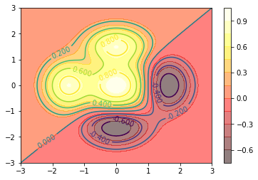
加上上面三行程式碼來修飾圖形,contourf()方法是用來著色,此處選擇的style為cmpa='hot'。clabel()會在線條上註解文字,選擇inline屬性使其顯示於線內,inline=0表連續線段。最後plt.colorbar()方法會產生一旁的對照尺,讓使用者觀察比對。
之前在介紹bar chart的時候提過若是要讓座標軸使用對數表示,可以讓參數log=True。不過在plot()與scatter()卻沒有這個屬性,所以若是想要使用對數顯示座標軸,可以使用如下方式:
x = np.arange(20) y = np.random.random(20)*10000 plt.plot(x,y) plt.yscale('log')
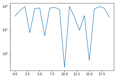
若是要顯示的是x軸,則使用plt.xscale()方法。若是使用ax=plt.subplot()而得到Axes物件,則可以使用
ax.set_xscale('log')或
ax.set_yscale('log')方法來設定。另一個方式是使用semilogy()方法,如下:
plt.semilogy(x,y,'bo')
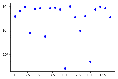
效果是完全相同的,只是這裡選擇使用散佈圖形式表現。很顯然若是要scale成為log的是x軸,那麼可以使用
plt.semilogx()雖然分別繪製x與y可以得到兩軸都是log scale的目的,不過較為便利的方式應該是使用loglog()方法,如下:
plt.loglog(x,y,'b-')
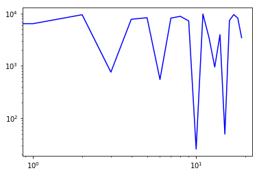
簡單方便。接下來再來談一下DataFrame,之前提過DataFrame可以直接呼叫plot()方法來繪製各式圖形,此處介紹其中的兩種選項,box與area圖形,舉例如下:
df1 = pd.DataFrame(np.random.randint(1,100,(10,3))) df1.plot(x=df1.index, y=[0,1,2], kind='box')
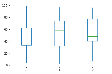
也可以使用
df1.plot.box(x=df1.index, y=[0,1,2])指令繪製,效果是相同的。而所顯示的資料是四分位數(quartiles),也就是25%、50%、75%等位數。可以使用describe()方法查看數值,例如:
df1[0].describe()另一個area圖形的做法則如下:
df1.plot(x=df1.index, y=[0,1,2], kind='area') #df1.plot.area(x=df1.index, y=[0,1,2]) plt.minorticks_on()
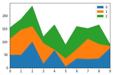
此方法可以繪製面積圖,也就是累加圖形,塗上面積顏色。使用plt.minorticks_on()方法來讓較小刻度顯現。與前相同,前兩行的兩種寫法任一都可以達到相同的效果。
與前述box圖形類似的是小提琴圖(violin plot),圖中可以顯示最大數、最小數、平均數、中位數、以及數字頻率,使用violinplot()方法,例如:
df = pd.DataFrame(np.random.randint(1,100,(10,10))) plt.violinplot(df[1], showmeans=True, showmedians=True)

第一個參數是輸入的資料(dataset),在此選擇df的一欄。設定showmeans與showmedians為True來顯示平均數與中位數。若設定vert=False則圖會翻轉90度。事實上可以直接給整個DataFrame資料,如此會直接針對每一欄進行violinplot的繪製,如下:
df = pd.DataFrame(np.random.randint(1,100,(10,10))) plt.violinplot(df, showmeans=True, showmedians=True, widths=0.8)
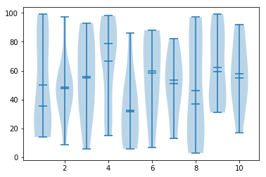
使用widths參數來控制寬度,可以讓圖形看起來更明瞭。在繪製圖形時,主要包含幾個物件,首先第一個是figure,這個物件代表的就是一個圖形顯示區,第二個就是axes,基本上這就是一個四方框讓我們畫一個圖,一個figure可以包含多個axes物件,這樣就形成了多圖,我們在第104話用過的subplots()方法就是可以傳回一個figure加上多個axes。在此我們討論如何取得這些物件來繪圖。首先看下例:
fig1 = plt.figure(num=1,figsize=(3,3), dpi=100,facecolor='lightgreen', edgecolor='blue', linewidth=3, frameon=True) ax1 = fig1.add_axes([0.1,0.1,0.8,0.8]) ax1.plot(df1[0], 'red', linewidth=1.5, linestyle=':')
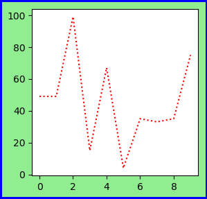
fig2 = plt.figure(num=2) ax2 = fig2.add_axes([0.1,0.1,0.8,0.8]) ax2.plot(df1[1]) ax2.plot(df1[2],color='green') ax2.legend()
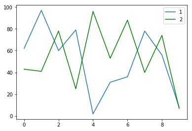
此處繪製兩個figure,所以是兩個圖形顯示區,其中的參數linewidth=3代表的是邊線的寬度,如果frameon=False,則facecolor與edgecolor等皆強制不顯示,而frameon的預設值為True。
這裡要提一下num這個參數,兩個figure的num不同,表示是不同的顯示區,那麼若是相同(例如將fig2的num改為1),那這三條折線會繪製在同一個顯示區內,也就是僅有一個顯示區。此外,dpi的預設值就是100,這個參數是解析度,如果把值加大,圖會比較清楚,不過原則上圖也會變大。
之前提及axes是一個圖,這個物件我們原則上不會自行宣告,主要靠兩個函數產生,其一是add_axes(),其二就是add_subplot()。回顧一下,若是使用pyplot的話還可以使用plt.gca()方法取得目前axes物件(106話)。而add_axes()其中的參數是一個list,四個數字代表left、bottom、width、height。寬高的值則會讓圖根據figsize()的大小依該值比例縮放。提醒一點,可以像之前學的方法一樣直接使用plt.plot()繪製,這個方法會直接作用到目前的axes。所以如果我們想要在一個figure中加入兩個axes,除了之前提過的多圖(使用add_subplot()),可使用add_axes()兩次,例如:
fig3 = plt.figure(num=1) ax1 = fig3.add_axes([0.1,0.1,1,1]) ax2 = fig3.add_axes([0.75,0.8,0.25,0.25]) ax1.plot(df1[0], 'red', linewidth=1.5, linestyle=':') ax2.plot(df1[0], linewidth=0.8)
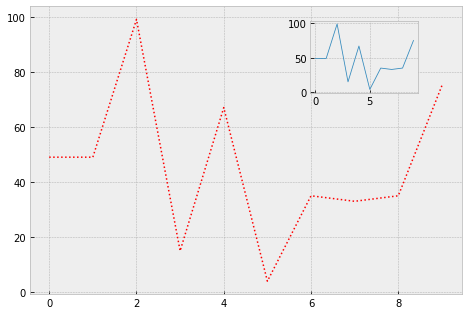
這個例子應該足夠鮮明地告訴我們add_axes()內的參數意義了。再看一個例子:
fig3 = plt.figure(num=1) ax1 = fig3.add_axes([0,0,0.5,1]) ax2 = fig3.add_axes([0.5,0,0.5,1]) ax1.plot(df1[0], 'red', linewidth=1.5, linestyle=':') ax2.plot(df1[1], linewidth=0.8)
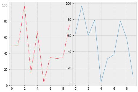
另一個使用雙軸的方式是利用twinx(),用來共享x軸,若是使用twiny()則是共享y軸。
fig4 = plt.figure(num=1) ax1 = fig4.add_axes([0.1,0.1,1,1]) ax2 = ax1.twinx() ax1.plot(np.random.randint(1,100,10), 'red', linestyle=':') ax2.plot(np.random.randint(100,1000000,10), 'blue') ax1.set_ylabel("df1[0]", color='red') ax2.set_ylabel("df1[1]", color='blue')
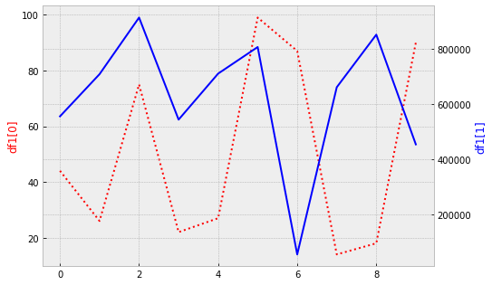
-
Talk112_1.py
- 使用plt.contour()方法來繪製等高線圖
- 使用plt.plot()+plt.yscale()、plt.semilogy()、plt.semilogx()、plt.loglog()等方法來建立以log為scale之軸
- 使用DataFrame.plot.box()方法繪製四分位圖
- 使用DataFrame.plot.area()方法繪製面積圖
- 使用plt.violinplot()方法繪製小提琴圖
- 使用fig=plt.figure()取得figure物件,並使用add_axes()或add_subplot()取得axes物件
Recap
第一百一十三話、matplotlib之3D圖形
如果要繪製3D的圖形,需要導入from mpl_toolkits.mplot3d import Axes3D。有這個3D軸,就可以畫3D的圖了,當然還是分散佈圖、折線圖、長條圖等類型,先看散佈圖的例子:import numpy as np import pandas as pd import matplotlib.pyplot as plt from mpl_toolkits.mplot3d import Axes3D np.random.seed(113) x1 = np.random.randint(10,20,50) y1 = np.random.randint(10,20,50) z1 = np.random.randint(10,20,50) x2 = np.random.randint(50,70,50) y2 = np.random.randint(50,70,50) z2 = np.random.randint(50,70,50) ax = Axes3D(plt.figure()) ax.scatter(x1,y1,z1,'bo',label="data 1") ax.scatter(x2,y2,z2,'r.',label="data 2") ax.set_xlabel('X') ax.set_ylabel('Y') ax.set_zlabel('Z') plt.title("3D Scatter",color='blue',fontsize=30) ax.legend(loc=0)
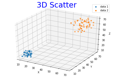
首先設計兩組資料,因為是3D,所以要有三軸的資料。宣告Axes3D(figure)需要一個figure作為參數。接下來直接使用scatter(x,y,z)來繪製即可,跟2D的用法差不多,一樣可以使用set_xlabel()與legend等方法。
如果要繪製3D長條圖,做法類似,使用的指令為bar3D(),舉例如下:
x = np.arange(5) y = np.arange(5) x, y = np.meshgrid(x,y) x, y = x.ravel(), y.ravel() z = np.random.randint(1,20,25) bottom = np.zeros_like(z) fig = plt.figure() ax = Axes3D(fig) ax.bar3d(x,y,bottom, dx=0.5,dy=0.5,dz=z, color='b', shade=True) ax.set_xlabel('X') ax.set_ylabel('Y') ax.set_zlabel('Z') ax.view_init(elev=60, azim=125)
此處的x、y、z數列都是1D,個數為25,使用np.meshgrid()只是要讓其都介於0-5之間。也可以使用np.random.randint()來產生x與y,只是要注意可能會有重複的點。再使用bar3d()時,前面三個參數為起始位置,而dx、dy、dz則為各向的長度,也就是柱體長寬高。Shade為True表示顯示陰影。ax.view_init()方法用來控制視角,elev與axim分別為高程跟方位。
這麼多長柱體可能會看不太清楚,所以也可以控制每根柱體的顏色皆不同,事實上可以控制每個柱體每一面的顏色都不同,因為需要很多顏色,所以先設計一個函數隨機產生顏色:
def genColor(): return [np.random.random() for i in range(3)]注意此方法與之前介紹的不同,這裡的顏色使用陣列[R,G,B]來表示,數值介於0~1之間。接下來只要將顏色修改如下:
ax.bar3d(x,y,bottom, dx=0.5,dy=0.5,dz=z, color=[genColor() for i in range(25)], shade=True)
因為每個柱體顏色都不同,所以要設計25種顏色。或是
ax.bar3d(x,y,bottom, dx=0.5,dy=0.5,dz=z, color=[genColor() for i in range(25*6)], shade=True)
此處因為每個柱體每一面的顏色都不同,所以要設計25*6種顏色。
接下來談繪製曲線圖,只要使用plot()方法並給x、y、z資料即可,例如:
x = np.arange(10) y = np.arange(10) z = np.random.randint(1,100,10) ax = Axes3D(plt.figure()) ax.plot(x,y,z,color='b')
plot()方法可以繪製2D與3D圖形。若是要繪製某些數學函數圖形,則跟之前介紹的2D畫法類似,給定小間隔的值來平滑曲線即可,例如:
theta = np.linspace(-10*np.pi, 10*np.pi, 300) z = np.linspace(-2,2,300) x = 2*z*np.sin(theta) y = 2*z*np.cos(theta) ax = Axes3D(plt.figure()) ax.plot(x,y,z,color='b')
也不困難,只要給定x、y、z的值即可繪製。有的時候我們想要給3D圖形加上表面,此時做法如下:
x = np.arange(-5,5,0.1) y = np.arange(-5,5,0.1) x, y = np.meshgrid(x,y) z = np.cos(2*np.sqrt(x**2+y**2)) fig = plt.figure() ax = Axes3D(fig) ax.plot_wireframe(x,y,z,rstride=1,cstride=1) surf = ax.plot_surface(x,y,z,cmap='hot') #fig.colorbar(surf, shrink=0.25, aspect=15) ax.set_xlabel("X") ax.set_ylabel("Y") ax.set_zlabel("Z") ax.view_init(elev=60, azim=125)
首先因為需要先使用ax.plot_wireframe()方法來繪製網格結構圖,其輸入的x、y、z資料需為2D的矩陣排列。方法中的rstride與cstride參數是表示row跟col的跨度,此值越小表示網格越密。接著使用ax.plot_surface()方法來繪製表面,可以使用color參數來設定參數,此處使用cmap來設定color map。而使用cmap的話便可以使用fig.colorbar()方法來顯示對應顏色尺。
-
Talk113_1.py
- 繪製3D圖形需導入from mpl_toolkits.mplot3d import Axes3D
- 產生3D軸需使用ax=Axes3D(figure)方法
- 使用ax.scatter()方法來繪製3D散佈圖
- 使用ax.bar3d()方法來繪製3D長條圖
- 使用ax.plot()方法來繪製3D曲線圖
- 使用ax.plot_wireframe()方法來繪製網架以及使用ax.plot_surface()方法來繪製表面圖
Recap
Python亂談
Seaborn
第一百一十四話、初談Seaborn
Seaborn是另外一套繪圖的模組,與matplotlib不大相同,主要用於統計資料的視覺化,可說是matplotlib的進階補充版。它有強大的功能讓我們很容易的繪製統計相關圖型。要使用seaborn顯然需要導入,以下列出所有要導入的模組:import numpy as np import pandas as pd import matplotlib.pyplot as plt import seaborn as sb先都導入,最後發現用不到再刪。為了方便說明並且順便回味一下之前的內容,在此使用交通部統計查詢網https://stat.motc.gov.tw/mocdb/stmain.jsp?sys=100查詢高雄捷運客運概況,選擇紅橘線的人次與延人公里,如下:
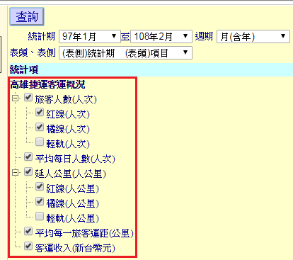
點選查詢後,資料會出現在此網頁。
要想取得這個網頁的資料,顯然需要使用read_html()方法,如下:
kmrt = pd.read_html("網址",header=0, index_col=0)[1]
因為上面的網址列很長,這裡使用網址替代,header=0表示第一行做為columns的名稱,index_col=0表示第一列做為index的名稱。那這個[1]是指?如果沒有加上這個[1],你會發現讀取這一頁得到的矩陣有兩個元素,第一個是標題的內容,第二個才是資料表格,所以加上[1]表示只要資料表格。
接下來仔細觀察資料,發現在每一年一開始都有一筆全年資料,然後才是各月的資料,我們只要各月資料,所以使用以下方式刪除各年資料:
kmrt = kmrt.drop(['97年','98年','99年','100年','101年','102年', '103年','104年','105年','106年','107年','108年(1月至2月)'])因為在繪圖時有時中文字顯示不出來,所以還是改為英文較好,此外,index是時間序列,也可以替換為時間為軸,所以處理如下:
newindex = pd.date_range(start='2008/4/30', periods=131, freq='M', name='Date') kmrt.index=newindex kmrt.columns = ['Passengers', 'RedLine', 'OrangeLine', 'DailyPassengers', 'PassengerKM','RedPassengerKM','OrangePassengerKM', 'AveKMperPassenger', 'Income']嗯,現在好多了,觀察一下資料,又發現橘線在2008年4月到8月並無資料,因為當時尚未通車,資料是使用-表示,我們可以將其替換為0,如下:
kmrt['OrangeLine'][0:5] = 0 kmrt['OrangePassengerKM'][0:5] = 0接著查看一下資料:
kmrt.head(10)不過改值後執行時會出現警告訊息,可以別理,若想省略它,加上以下指令:
import warnings warnings.filterwarnings('ignore')看起來好多了。
之前提過seaborn可以用來補足matplotlib,而且seaborn繪出來圖不同(有人覺得比較美,看個人喜好),我們可以直接將matplotlib的圖轉換成seaborn的圖,只要加上
seaborn.set(context='notebook', style='darkgrid', palette='deep', font='sans-serif', font_scale=1, color_codes=True, rc=None)這個方法即可,如下:
sb.set() kmrt.plot()
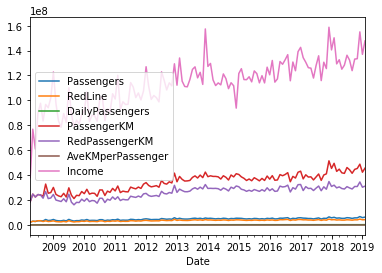
|
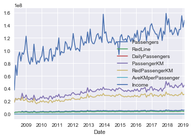
|
- Context: 此參數定義內容文字大小,可以選擇的值自小到大有paper、notebook(預設值)、talk、poster。文字大小也可以使用font_scale參數來改變(例如: font_scale=2)。例如:
sb.set(context="poster", font_scale=0.5)
也可以使用sb.set_context(context='poster', font_scale=0.5)
方法替代。 - Style: 控制背景顯示風格,可以選擇的值有darkgrid(預設值)、whitegrid, dark、white、ticks。也可以使用
sb.set_style("whitegrid")
替代。例如:sb.set(context='paper', style='whitegrid') #sb.set_style("whitegrid") kmrt.plot()
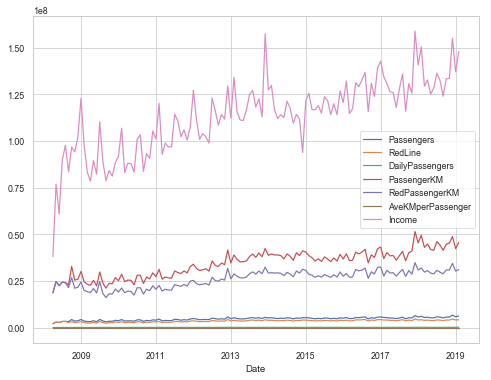
若是使用dark或是white則沒有格線(grid)。 - Palette: 用來控制色調。Seaborn色調可以選擇的值為deep、muted、bright, pastel、dark、colorblind,此外,也可以使用之前提過的cmap的值,例如hot。也可以使用
sb.set_color_codes(palette='muted')
方法設定。例如:sb.set(context='paper', style='darkgrid', palette='hot') #sb.set_color_codes(palette='muted') kmrt.plot()
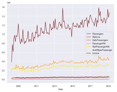
選擇了palette後,在繪製時便不要指定顏色(例如使用kmrt.plot(color='r')),否則會將palette的配色蓋過。 - rc: 其值為一dict,可用來控制上述的參數。例如:
rc={'figure.figsize':(8,6), 'lines.linewidth':2}
表示設定圖的大小與其中線的寬度。在sb.set_style()中也有rc這個參數,在此方法中則為設定軸的參數。sb.set(context='paper',palette='winter', rc={'figure.figsize':(8,6), 'lines.linewidth':2}) #sb.set_context(context='paper', rc={'lines.linewidth':2}) sb.set_style('whitegrid', rc={'ytick.color': 'red'}) kmrt.plot()

set_context()方法中也可以加上rc參數來改變內容。注意改變內容的rc跟改變軸內容的rc並不相同。
關於軸的參數,可以輸入print(sb.axes_style())
來看到相關內容。
-
Talk114_1.py
- 欲使用seaborn須先導入import seaborn as sb
- 使用sb.set()來將圖形改由seaborn繪製
- 控制sb.set()內的參數包括context、style、palette、rc等來改變圖形外觀
Recap
第一百一十五話、Seaborn之relplot()
上一話提到如何設定seaborn的繪圖風格,此處來談如何使用seaborn繪圖指令。除了修改matplotlib的繪圖風格使其成為seaborn圖形,seaborn也有自訂的繪圖功能指令。在此介紹使用relplot()方法(relational plot),此方法可以直接繪製DataFrame的內容,只要設定最主要的三個參數,x、y、data,如下:sb.set(context='paper',style='darkgrid',palette='hot') sb.relplot(x='Passengers',y='Income',data=kmrt)
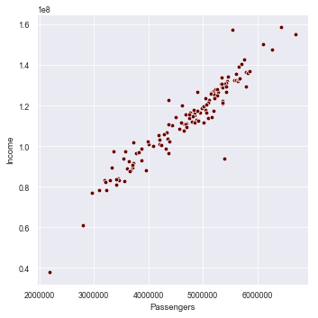
此處x與y接受字串,且須為kmrt內的columns名稱。使用relplot()若沒有加上sb.set()則繪圖使用預設值。原則上到目前與使用
plt.plot(kmrt.Passengers, kmrt.Income, 'b.')沒太多差別。
上圖的資料點看起來都一樣,如果其中有因素可將其分類,我們可以使用hue來讓它們用不同顏色顯示,例如:
sb.set(context='paper',style='darkgrid') sb.relplot(x='Passengers',y='Income', hue='AveKMperPassenger',palette='hot', data=kmrt, height=6, legend='brief')
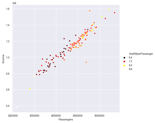
因為relplot()就有palette屬性參數,所以便不再在set()內設定。使用height可以定義圖的高度,可藉此調整圖的大小。
此處使用AveKMperPassenger來做為hue的基礎,可是細看資料的話,每行的AveKMperPassenger並不相同,所以若是我們將legend的值換成full,將會看到一大排的圖示。通常最好是有資料能將數據區分為少數幾類,例如:
kmrt['eo'] = ['Odd' if i.month%2 else 'Even' for i in kmrt.index] sb.set(context='paper',style='darkgrid',palette='bright') sb.relplot(x='Passengers',y='Income', hue='eo',palette=['b','r'],style='eo', data=kmrt, legend='brief')
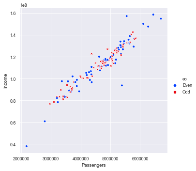
首先在kmrt內加上一欄名為eo表示月份的單雙,如此可將資料分為兩類。將palette設定為兩色的list,之後便利用這兩色來著色。因為色調是自己設計的,不是來自調色好的cmap,所以再回頭到set()內設定palette為bright,如此可讓顏色調整為亮度較高的色調。除此之外,再加上設定style為eo表示圖的顯示除了顏色不同,連形狀也依不同群組而有所不同,hue跟style不需要設為相同,如果有其他分類方式的話,兩者可以設為不同,例如:
kmrt['eo'] = ['Odd' if i.month%2 else 'Even' for i in kmrt.index] def season(x): if x <= 3: return 1 elif x <= 6: return 2 elif x <= 9: return 3 else: return 4 kmrt['season'] = [season(i.month) for i in kmrt.index] sb.set(context='paper',style='darkgrid',palette='bright') sb.relplot(x='Passengers',y='Income', hue='eo',palette=['b','r'],style='season', data=kmrt, legend='brief', size='season')
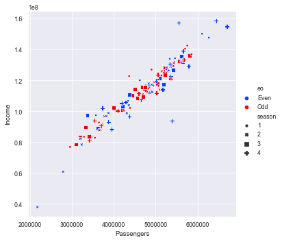
此處將資料又區分為四季,每一季使用不同的形狀。要注意分類數有限制,過多的組別會出現錯誤。事實上上例中還有一個分類描述是size,從legend也可以看出來,圖上的點依次自1到4漸次增大。其實我們還可以進一步控制點的大小,只要加上sizes=(5,50)就表示點的大小範圍為5到50,請自行嘗試。
除了使用relplot()方法之外,也可以使用scatterplot()方法來繪製,將上例的relplot()替換為scatterplot()如下:
sb.scatterplot(x=kmrt.Passengers,y=kmrt.Income, hue='eo',palette=['b','r'], style='season', data=kmrt, legend='brief', size='season', sizes=(5,50), alpha=0.6)
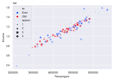
圖的樣式有點不同(Legend在圖內),其餘效果原則上都相同。
事實上還是有些微不同,上例的x、y可以輸入一維陣列形式的資料(當然也可以是columns的名字),但是在relplot()中若是輸入一維陣列資料則會出現錯誤。若是資料不是使用DataFrame形式的情況下,scatterplot()還是可以輕鬆的繪製圖形,例如:
xy = np.random.randint(1,100,(2,100)) sb.set(context='paper',style='darkgrid', palette='magma') sb.scatterplot(x=xy[0],y=xy[1])
 雖然這樣也行,不過因為seaborn的功能可以很好的跟Pandas資料結構搭配,所以把資料儲存成DataFrame再來繪製似乎是個好主意。
接著來看折線圖的畫法,原則上還是使用relplot()方法,只是將kind設定為line,例如:
sb.set(context='paper',style='darkgrid',palette='bwr') sb.relplot(x='Passengers',y='Income',data=kmrt, kind='line')
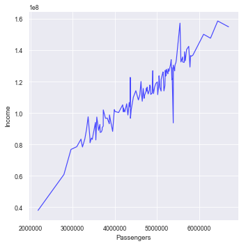 原則上跟之前介紹的參數用法都相同,只是將kind改為line。這個圖在某些領域中可以讓我們看出趨勢,例如股票走向。跟散佈圖類似,除了使用relplot()之外,也可以使用lineplot()這個方法來繪製折線圖,請自行練習。
上例的圖其實是排序過的,因為這裡預設我們想要根據排序過後的x軸資料來繪製,若是這不是我們想要的結果,可以加上sort=False來取消排序,也請自行練習。因為參數都類似,所以直接修改前例來練習繪製曲線圖,此處我們想要知道每一季的收入趨勢,做法如下:
kmrt['date'] = kmrt.index kmrt['season'] = [season(i.month) for i in kmrt.index] sb.set(context='paper', style='darkgrid', palette='bright') g = sb.relplot(x='date', y='Income', hue='season', palette=['b','r','g','k'], style='season', data=kmrt, legend='brief', size='season', sizes=(0.5,2), height=8, kind='line',markers=True) g.fig.autofmt_xdate()
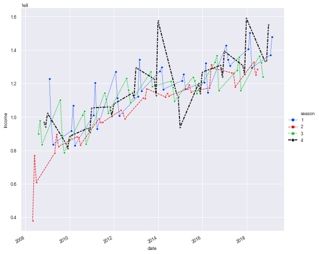 新加入一欄為date,取自index。當然還是可以使用lineplot(),不過得去除掉部分參數,例如height與kine。
上圖中額外加上markers=True來讓每個點顯示出來,此外,若是不想要虛線,可以加上dashes=False。因為x軸是日期時間,所以還可以加上g.fig.autofmt_xdate()方法來協助顯示日期。若是想要將上例分為多個圖形顯示,則加上col參數並將其值設定為season即可,顯示結果如下:
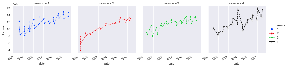
-
Talk115_1.py
- 使用sb.relplot()或sb.scatterplot()來繪製散佈圖
- 使用sb.relplot(kind='line')或sb.lineplot()來繪製折線圖
- 使用參數hue、style、與size&sizes來顯示資料的不同群組且可使用col參數來繪製subplot
Recap
第一百一十六話、Seaborn之catplot()
對於數值統計來說,可以描繪分類觀察點的分布及密度的圖表等可以讓我們很容易地看出一些趨勢,所以接下來介紹catplot()這個方法(Categorical plot)。此方法可以讓我們繪製類別資料,而類別資料又可以分為三種圖,分別為散佈圖(scatter plot)、分配圖(distribution plot)、估量圖(estimate plot)。我們一樣採用之前的高雄捷運人次資料。這裡的散佈圖跟之前介紹的略有不同,此處是根據不同類別來繪製資料,例如:
sb.set(context='paper',style='darkgrid') sb.catplot(x='season',y='Income',data=kmrt,kind='strip',hue='eo',palette='hot',legend_out=False)
 這裡顯示每一季的收入情況,每一季中還分單雙月以不同顏色顯示。加上legend_out=False的設定,可以讓legend在圖內顯示。這裡的kind設定為strip,就是繪製散佈圖的意思,是此方法的預設值。
跟之前的relplot()方法一樣,不同的kind也有對應不同的方法,此處為stripplot()方法。只要使用
sb.stripplot(x='season',y='Income',data=kmrt,hue='eo',palette='hot')替代catplot()即可,請自行嘗試。另一種顯示方式是設定參數jitter=False,如此每一類別的點會擠在一線上,例如:
sb.set(context='paper',style='darkgrid') sb.catplot(x='season',y='Income',data=kmrt,jitter=False, hue='eo',palette='gnuplot',legend_out=False)
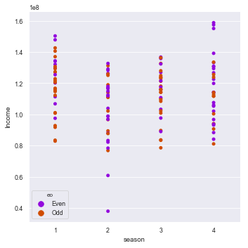 其他參數的配置都類似。也可以在stripplot()中設定jitter參數。
之前介紹的散佈圖難免會有點重疊的情形,若是不想出現重疊,則可以使用kind=swarm來繪製散佈圖,例如:
sb.set(context='paper',style='darkgrid') sb.catplot(x='season',y='Income',data=kmrt,kind='swarm',hue='eo',palette='gnuplot',legend_out=False)
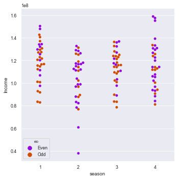 由上圖可看出點並不重疊。同樣的,也可以使用swarmplot()方法來繪製相同的圖形。我們甚至可以過濾掉部分不想顯示的資料,只要在給定data時給條件即可,例如:
sb.set(context='paper',style='darkgrid') sb.catplot(x='season',y='Income',data=kmrt.query('season!=2'), kind='swarm',hue='eo',palette='brg',order=[4,1,3], legend_out=False)
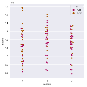 跟前例主要的不同在於data使用query()方法濾過,所以僅顯示三組資料。一樣的方式也可以應用到swarmplot()上。因為有固定組別,所以可以加上order=[4,1,3]設定讓顯示的順序改變。
以上這兩類是屬於散佈型態的圖,接下來介紹資料分配圖,主要的種類(kind)有box、boxen、violin三種。首先看box,如下:
sb.set(context='paper',style='darkgrid') sb.catplot(x='season',y='Income',data=kmrt,kind='box',hue='eo', palette='ocean', legend_out=False,dodge=False)
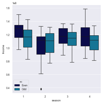 一樣可以使用boxplot()方法來繪製這個圖。這些box預設彼此會錯開避免重疊,若是不在乎是否重疊,可以設定dodge=False,請自行練習。
第二種圖形為boxen,只要改變kind即可,如下:
sb.set(context='paper',style='darkgrid') sb.catplot(x='season',y='Income',data=kmrt,kind='boxen', hue='eo',palette='prism', legend_out=False)
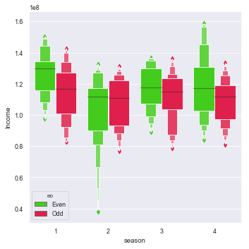 Boxen圖形是強化版的box,有利於大筆資料的描繪。一樣可以使用對應的boxenplot()來繪製。
第三種是小提琴圖,一樣簡單容易,直接繪製如下:
sb.set(context='paper',style='darkgrid') sb.catplot(x='season',y='Income',data=kmrt, kind='violin', legend_out=False, hue='eo',palette='nipy_spectral_r')
 也可以使用violinplot()方法來繪製相同的圖。小提琴圖有其他花樣可供選擇,譬如說將單筆資料標註成線,做法是設定inner參數,可供選擇的值有box、quartile、point、stick、None。
在此額外設定split=True,讓其在中間使用分隔線,若是設定split=False則回復上例之分開型態。
sb.set(context='paper',style='darkgrid') sb.catplot(x='season',y='Income',data=kmrt, kind='violin', legend_out=False, hue='eo',palette='nipy_spectral_r', split=True, inner='stick', height=5, aspect=1.1)
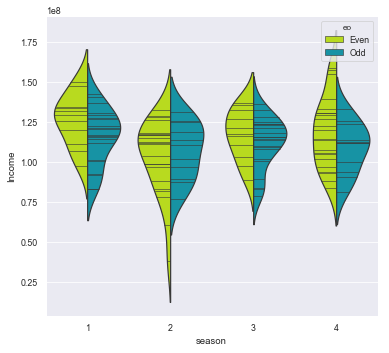 使用height來設定高度(inches),而寬度則等於height*aspect。
以上介紹這三種圖總稱為資料分配類型的圖,可以讓我們觀察資料的分配情況。我們其實可以將散佈圖與資料分配圖畫在一起合成一個圖,只要一個使用catplot()而另一個使用替代方法即可,例如:
sb.set(context='paper',style='darkgrid') g = sb.catplot(x='season',y='Income',data=kmrt, kind='violin', legend_out=False, hue='eo',palette='coolwarm', split=True, inner='stick', height=5, aspect=1.1) sb.stripplot(x='season',y='Income',data=kmrt, hue='eo',palette='hot') g.set_xticklabels(["Q1", "Q2", "Q3","Q4"])
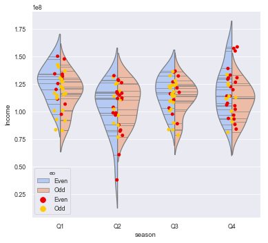
最後一類是估量圖,包含bar、count、與point三種類型。畫法都是類似,只要修改kind即可,首先看bar的畫法,舉例如下:
sb.set(context='paper',style='darkgrid') g = sb.catplot(x='season',y='Income',data=kmrt, kind='bar', legend_out=False, hue='eo',palette='coolwarm', height=5, aspect=1.1) g.set_xticklabels(["Q1", "Q2", "Q3","Q4"])
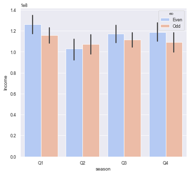 對應的替代方法為barplot()。再來看count plot,例如:
sb.set(context='paper',style='darkgrid') g = sb.catplot(x='season',data=kmrt, kind='count', legend_out=False, hue='eo',palette='gist_ncar', height=5, aspect=1.1) g.set_xticklabels(["Q1", "Q2", "Q3","Q4"])
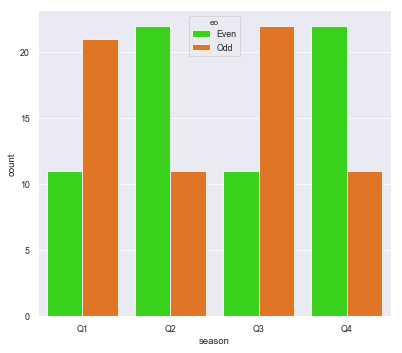 對應的替代方法為countplot(),顯示圖形也是一個長條圖,若想橫向,將x修改為y即可。
這個例子雖然順利的繪出圖形,不過涵義乏善可陳,因為在計數的是season個數,不過因為例子中並無適合計數的資料,只好用season表示。若有資料會重複出現,譬如性別或職業等,即可使用此方法來計數。
最後看point plot的做法,舉例如下:
sb.set(context='paper',style='darkgrid') g = sb.catplot(x='season',y='Income',data=kmrt, kind='point', legend_out=False, hue='eo',palette='PuRd', height=5, aspect=1.1) g.set_xticklabels(["Q1", "Q2", "Q3","Q4"])
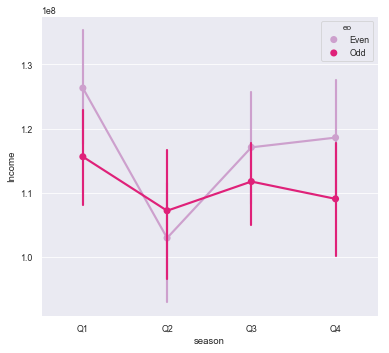 類似的情況,對應的替代方法為pointplot()。這裡的圖都是直立的,若是要繪製橫向的圖,可以加上orient='h'設定,然後讓x、y的值對調即可,唯一的例外是count plot,它只要將x改為y即可。以前述的兩圖同繪為例:
sb.set(context='paper',style='darkgrid') g = sb.catplot(y='season',x='Income',data=kmrt, kind='violin', legend_out=False, hue='eo',palette='coolwarm', split=True, inner='stick', height=5, aspect=1.1, orient='h') sb.stripplot(y='season',x='Income',data=kmrt, hue='eo',palette='hot', orient='h') g.set_yticklabels(["Q1", "Q2", "Q3","Q4"])
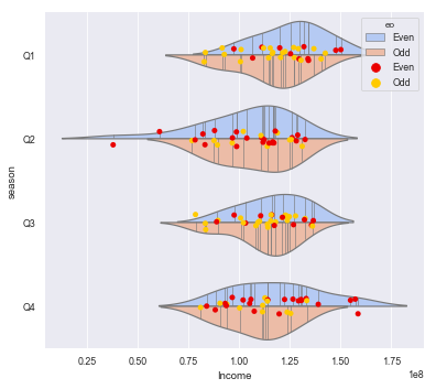
-
Talk116_1.py
- 使用sb.catplot(kind='strip') or sb.stripplot()來繪製類別散佈圖
- 使用sb.catplot(kind='swarm') or sb.swarmplot()來繪製不重疊之類別散佈圖
- 資料分配的圖形可使用sb.catplot(kind='box')、sb.catplot(kind='boxen')、sb.catplot(kind='violin')等方法來繪製
- 估量圖形可使用sb.catplot(kind='bar')、sb.catplot(kind='point')、sb.catplot(kind='count')等方法來繪製
Recap
第一百一十七話、Seaborn之分配圖
前述的seaborn功能好像並沒跳脫太多matplotlib的範疇,這裡來討論分配圖,與matplotlib會有較多區別,首先先看單一變數(univariate)的做法,當然還是繼續使用高雄捷運的例子,舉例如下:sb.set(context='paper',style='darkgrid') sb.distplot(a=kmrt.Passengers, bins=50, hist=True, kde=True, rug=True, # hist:長條圖、kde:gaussian kernel density estimate、rug:地毯圖 color='blue', vertical=False)
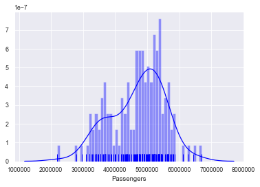 首先要注意此處須提供一個list-like的資料(list、Series等),參數名稱為a(在matplotlib中的hist()為x)。跟matplotlib中的hist()類似可以提供bins,而此處可以繪製hist(就是圖中的長條圖)、kde(gaussian kernel density estimate,就是曲線圖)、與rug(在最下方的地毯圖),你可以自己選擇要顯示哪幾個,只要給True或False的值即可。而vertial參數可以控制圖形是直立或是橫向。
我們可以根據不同參數的配置而得到不同類型的圖形,以下介紹幾種例子,將幾種圖繪製在一個subplots,如下:
f, axes=plt.subplots(2,2,figsize=(10,8)) sb.set(context='paper',style='darkgrid') sb.distplot(a=kmrt.Passengers, bins=50, hist=True, kde=True, rug=True, color='blue', vertical=False, rug_kws={'color':'g'}, kde_kws={'color':'r','lw':3,'label':"KDE"}, hist_kws={"histtype":"stepfilled", 'lw':3, "alpha":0.7, 'color':"#ff00ff",'label':"HIST"}, ax=axes[0,0]) sb.distplot(a=kmrt.Income,hist=False,color='red', kde_kws={'shade':True},ax=axes[0,1]) sb.distplot(kmrt.RedLine,kde=False,ax=axes[1,0], hist_kws={"histtype":"bar", 'color':"#ffff00"}) sb.distplot(kmrt.PassengerKM, hist=True, rug=True, color='k',ax=axes[1,1], hist_kws={"histtype":"step", 'color':"#5827f2"}) plt.tight_layout()首先使用subplots(2,2)來設計擁有2x2子圖的圖形,其軸為axes。然後繪製四個圖,利用ax這個參數,分別將圖放置於axes[0,0]、axes[0,1]、axes[1,0]、axes[1,1]四個位置(如果是兩個圖,例如subplots(2,1),那麼使用ax=axes[0]與ax=axes[1]來表示兩圖位置,如果僅有一個圖,那麼不需要設定ax,但還是可以使用plt.subplots(figsize=(10,8))來控制圖的大小)。
此外,可以利用kde_kws、hist_kws、與rug_kws三個dict來定義對應圖形的顯示屬性,例如lw為線寬,shade為陰影。Histtype用來顯示hist圖形型態,若是step為長條圖的外框線,bar為長條,stepfilled為填滿之step等。而tight_layout()的功能是自動調整圖形間距。顯示結果如下:
 這裡有兩個替代函數可以使用,分別為kdeplot()與rugplot(),顧名思義當然就是繪製kde與rug的方法,以下將兩種圖繪製在一起。
sb.kdeplot(data=kmrt.Passengers, shade=True, vertical=False, cumulative=False, color='blue') sb.rugplot(a = kmrt.OrangeLine, color='orange',height=0.05) sb.rugplot(a=kmrt.RedLine, color='red', height=0.08)
 在kdeplot()內若是將cumulative設為True,則為累加圖。在rugplot()中使用height來定義rug的高度,並可使用不同顏色(color)表示。事實上kdeplot()是可以繪製雙變數(bivariate)圖形的,例如:
sb.kdeplot(data=kmrt.RedLine, cbar=True, data2=kmrt.OrangeLine, shade=True,color='green') sb.rugplot(a = kmrt.OrangeLine, axis='y', color='orange',height=0.05) sb.rugplot(a=kmrt.RedLine, color='red', height=0.08)
 設定cbar=True來加上顏色對照軸。一樣將rugplot()繪製在一旁,使用axis參數來定義要繪製rug的軸。若是想要讓顏色更有變化,可以不使用color參數,直接設定cmap參數即可,你一定知道有哪些值可以使用。
事實上要繪製雙變數圖形,我們還有另一強大的選擇,也就是使用jointplot(),例如:
sb.set(context='paper',style='darkgrid') sb.jointplot(x="Passengers", y="Income", data=kmrt, kind='scatter', color='blue', height=8, ratio=5, space=0.2, s=50, edgecolor='y', linewidth=2, marginal_kws={'bins':30, 'rug':True, "rug_kws":{'color':'g'}, "hist_kws":{'color':'red'}})
 x與y也可以給list-like的值。中間的圖稱為joint而兩側的圖稱為marginal, 用以表示其分配。
參數height指的是整個圖的高度(圖為正方形),ratio指的是joint高度與marginal高度的比值,而space則是指joint與marginal的間距。而marginal_kws顯然就是控制marginal圖形的定義。繪製散佈圖使用kind的值為scatter,此為預設值,其他尚可選擇"reg"、"resid"、"kde"、"hex"等,只要修改kind的值即可繪製,例如:
sb.set(context='paper',style='darkgrid') sb.jointplot(x="Passengers", y="Income", data=kmrt, kind='hex', color='blue', height=8, ratio=5, space=0.2, edgecolor='y', linewidth=2, marginal_kws={'bins':30, 'rug':True, "rug_kws":{'color':'g'}, "hist_kws":{'color':'red'}})
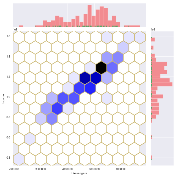 要注意並非所有參數都相同,例如此處並不s參數,請根據程式提示自行斟酌刪減。
若是要疊加其他圖形於jointplot(),再此不能僅同時繪製其他圖形,而是需要使用plot_joint()方法,做法如下:
sb.set(context='paper',style='darkgrid') g = sb.jointplot(x="Passengers", y="Income", data=kmrt, kind='kde', color='blue', height=8, ratio=5, space=0.2) g.plot_joint(sb.scatterplot,color='silver', s=5, marker='D')
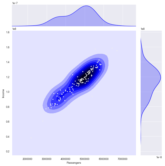 第一個參數需為一可呼叫的繪圖函數,sb.scatterplot或是plt.scatter之類,且此函數前兩個參數需是接受一維list-like值的參數。這個函數的圖會畫在跟joint plot相同的軸上。
-
Talk117_1.py
- 使用distplot()來繪製單一變數分配圖,替代方法包含kdeplot()與rugplot()
- 使用jointplot()繪製雙變數分配圖,也可以使用kdeplot()來繪製
- jointplot()的kind包含scatter、reg、resid、kde、hex等
- 疊加其他圖形於jointplot()需使用plot_joint()方法
Recap
第一百一十八話、Seaborn之迴歸圖
其實上一話介紹的jointplot()就可以繪製迴歸線,只要設定kind為reg即可,例如:sb.set(context='paper',style='darkgrid') sb.jointplot(x="Passengers", y="Income", data=kmrt, kind='reg', color='blue', height=8, ratio=5, space=0.2, marginal_kws={'bins':30, 'rug':True, "rug_kws":{'color':'g'}, "hist_kws":{'color':'red'}})
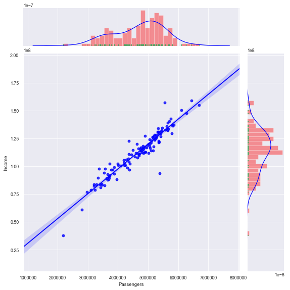 在上一話中已有完整介紹,此處不多贅述,看來旅客數與收入形成強烈相關。
迴歸的替代方法為regplot(),
sb.set(context='paper',style='darkgrid') sb.regplot(x="Passengers", y="Income", data=kmrt, x_bins=50, x_ci=None, scatter=True,fit_reg=True,ci=99, order=1, color='blue', marker="D", scatter_kws={'s':20,'color':'green'})
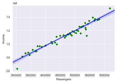 設定fit_reg為True會繪製迴歸線,此處order為1表示是一次關係。ci指的是信賴區間(confidence interval)。若是要控制圖的大小,跟之前介紹的方法類似,先使用f, axes=plt.subplots(figsize=(10,6))方法取得軸的控制,然後在方法中讓ax=axes即可。
另一個做法是使用lmplot(),原則上跟regplot()類似,只是lmplot()更進一步融合FacetGrid()的特點,舉例說明:
sb.set(context='paper',style='darkgrid') sb.lmplot(x="Passengers", y="Income", data=kmrt, x_bins=50, x_ci=None, scatter=True,fit_reg=True,ci=99, order=1, hue='season', markers=['o','x','+','D'], palette='Set1',scatter_kws={'s':20})
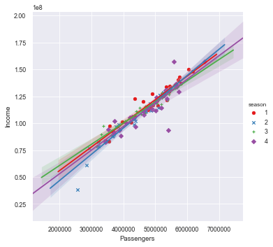 只要設定hue參數,可以很容易地分析不同組別資料的迴歸。
若是覺得所有圖都擠在一起,可以使用之前學過的col參數,設定為'season'則會繪製成四個圖(此時四個圖會排成一行,若是想要讓其排列具固定的欄數,譬如2列,則使用col_wrap=2)。甚至可以再加上row參數(例如row='eo'),如此可以根據不同組別繪製更多的圖(注意此時不能再使用col_wrap參數),結果如下圖:
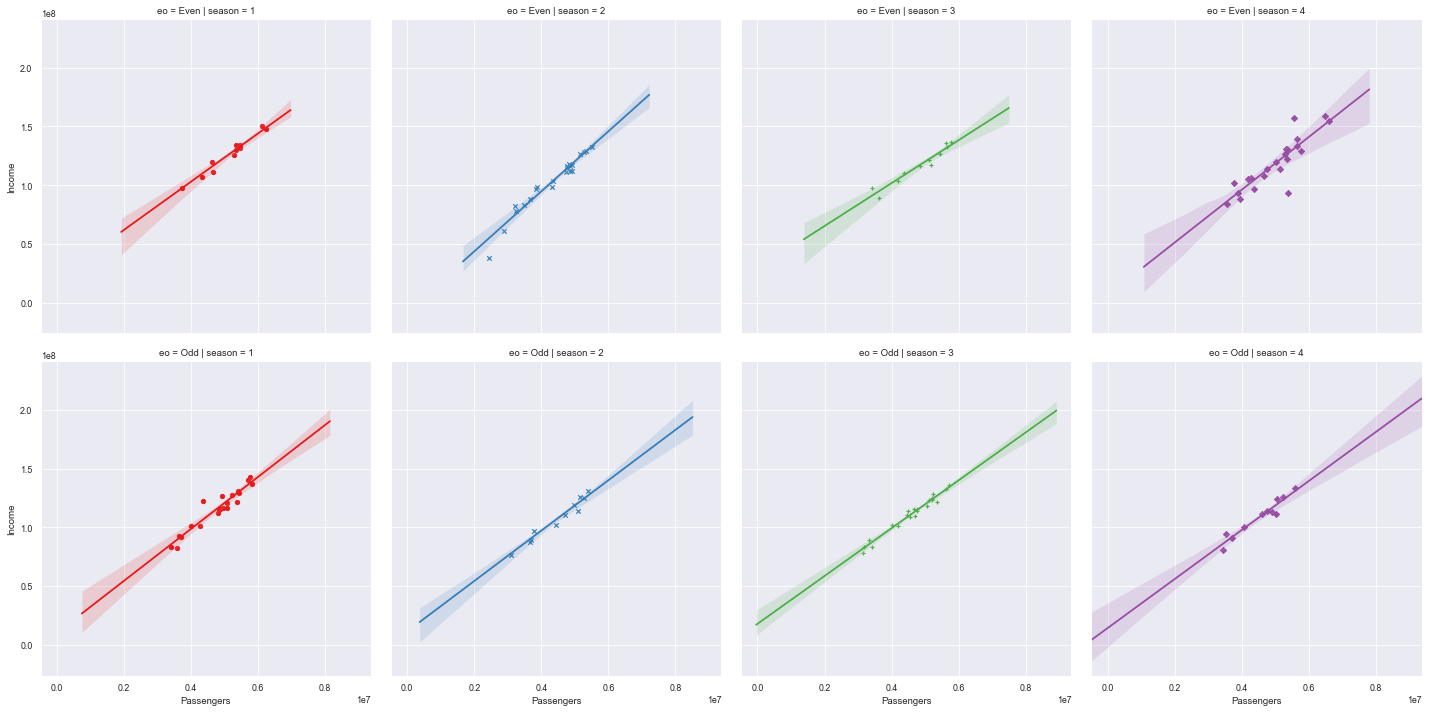 若是要控制圖的大小,使用height參數(e.g. height=5),此時圖形為正方形,若是要改變寬度,使用aspect參數(e.g. aspect=1.2)。
另一個統計相關圖形為殘差圖(residuals plot),使用residplot()方法,此方法會先算出y對x的迴歸式,然後計算殘差並繪製成散佈圖。例如:
sb.set(context='paper',style='darkgrid') sb.residplot(x="Passengers", y="Income", data=kmrt, order=1, color='blue', scatter_kws={'s':20})
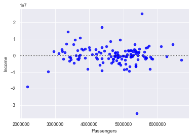 殘差的定義是r = y – ŷ,詳情請參考統計課本。此處可加上
f,axes=plt.subplots(figsize=(8,6))來控制圖形大小,你應該不陌生。之前使用過的jointplot()也可繪製殘差圖,各位應該有印象,只要設定kind的值為resid即可,請自行練習。
-
Talk118_1.py
- 變數的使用及計算
- 字串使用*號表示複製次數
- True(1)與False(0)首字母需大寫
Recap
第一百一十九話、Seaborn之多圖
之前提到的控制多圖的參數例如row、col、col_wrap以及控制圖案大小的height、aspect等參數適用於relplot()、catplot()、與lmplot()。而它們能夠繪製多圖原則上是因為根源於內含FacetGrid()方法。所以這裡來看看怎麼使用FacetGrid(),先舉例如下:sb.set(context='paper',style='darkgrid') grid = sb.FacetGrid(kmrt, col='season', col_wrap=2, hue='eo', palette='Set2', legend_out=False, height=5, aspect=1.2, hue_kws={'marker':['o','v']}) grid.map(sb.scatterplot, 'Passengers', 'Income', edgecolor='k') grid.add_legend()
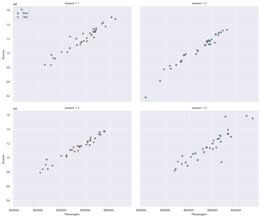 FacetGrid()方法的第一個參數是data,需為一DataFrame。跟之前介紹過的relplot()、catplot()、與lmplot()等用法類似,使用col與col_wrap來控制子圖布置,或使用row與col,row與col_wrap不能同時使用,看起來很面熟,那是因為本來就是同一件事情。
布置好了之後,使用map()方法繪製圖形製入,第一個參數是可呼叫的繪圖函數(例如scatterplot()或是plt.scatter()或plt.hist()等),之後是其所需參數。如果是要繪製relplot()、catplot()、與lmplot()等函數,因為其本身就可使用多圖,便不該再使用FacetGrid()方法。
另一個編織多圖的方式是使用PairGrid()方法,此方法的子圖座標包含不同變數,如此可以繪製每兩兩變數之間的關係圖。舉例說明:
sb.set(context='paper',style='darkgrid') grid = sb.PairGrid(kmrt, vars=['Passengers','Income'], hue='season',palette='Set2', height=5, aspect=1.2, hue_kws={'marker':['D','o','v','+']}) grid.map_diag(plt.hist) grid.map_offdiag(sb.scatterplot) grid.add_legend()
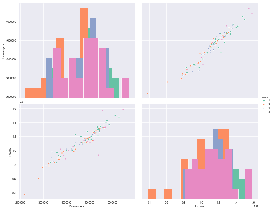 此處的grid使用PairGrid()來設定,因為kmrt包含很多的欄,都用的話會畫出很多圖,所以使用vars參數選擇其中兩個來繪製。接著一樣可以使用map()方法來繪製圖形置入,若是想要讓對角線的圖使用其他方法繪製,使用map_diag()方法,而非對角線的圖則使用map_offdiag()方法即可,如上例。除此之外,還可以根據對角線分為上部與下部,例如將map_offdiag()修改為如下:
grid.map_upper(sb.lineplot) grid.map_lower(plt.scatter) grid.map_diag(plt.hist)
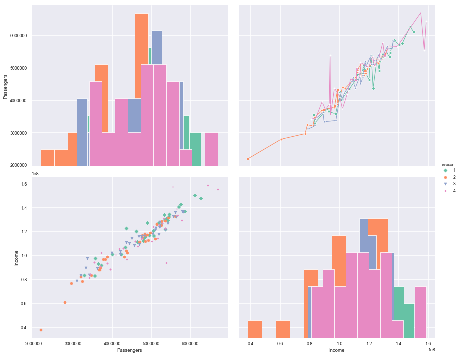 map_lower()方法繪製對角線下部的圖,而map_upper()方法繪製對角線上部的圖。
另一個分圖的方式是利用設定x_vars與y_vars參數(與設定vars的方式類似),繪製出兩軸排列組合的圖形,例如:
sb.set(context='paper',style='darkgrid') grid = sb.PairGrid(kmrt, x_vars=['DailyPassengers', 'AveKMperPassenger'], y_vars=['Income'], hue='season',palette='Set2', height=5, aspect=1.2, hue_kws={'marker':['D','o','v','+']}) grid.map(sb.regplot) grid.add_legend()
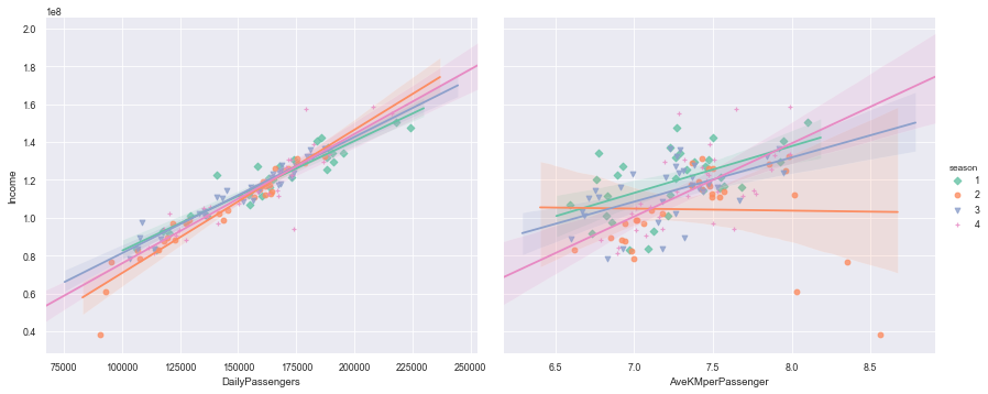 也可以直接使用對應方法pairplot()來繪製,做法如下:
sb.set(context='paper',style='darkgrid') grid = sb.pairplot(kmrt, vars=['DailyPassengers','Income'], hue='season',palette='Set2', height=5, aspect=1.2, markers=['D','o','v','+'], diag_kind='hist', kind='scatter') grid.add_legend()
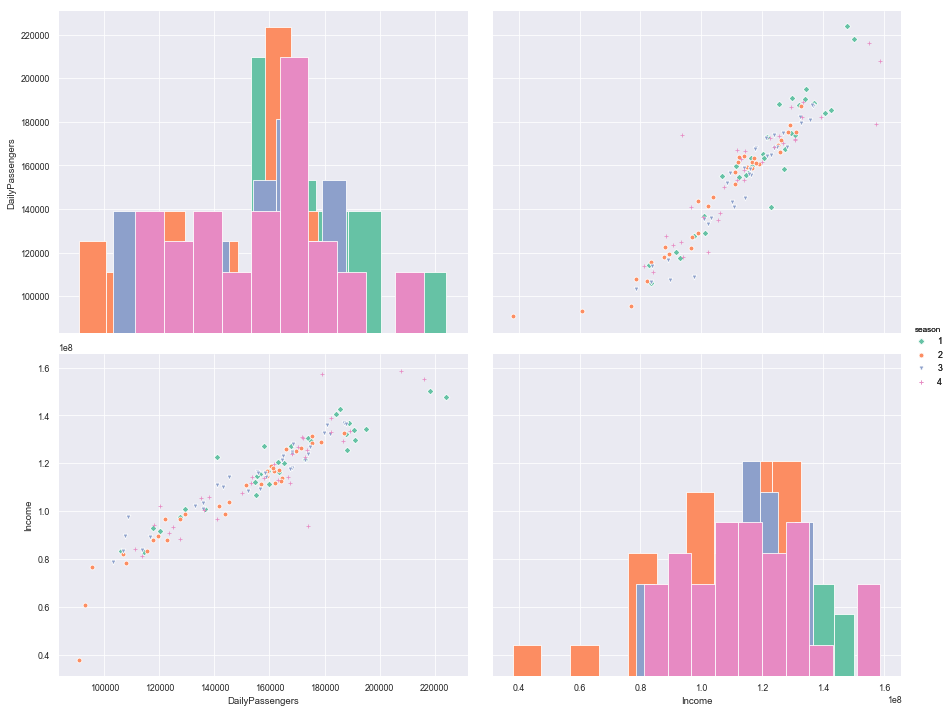 一樣也可以設定x_vars與y_vars來定義子圖座標。此處的kind可以使用的選擇包含scatter、reg,而diag_kind可以使用的選擇包含auto、hist、kde,看來選擇性是差了點。
Seaborn繪圖的方法就聊到這裡,順帶一提的是一直使用的數據kmrt,我們應該在第一次建立成完整DataFrame後,儲存在檔案、sql、或是pickle等處,如此便不需要每次都連到網站萃取資料,僅需做一次即可,不過我想各位應該都有閃過這個念頭,在此再次提醒。此外,我們可以使用sb.get_dataset_names()來查詢網路上可用的資料庫名稱,此時當然需要有網路,然後再使用例如
ans = sb.load_dataset('anscombe ')來讀取,之後可以直接使用其中資料繪圖,原則上讀到的便是一個DataFrame,若自己沒資料可使用時可以方便練習。再者,除了matplotlib與seaborn之外,還有其他繪圖方法例如Bokeh,有興趣可以自行練習。
-
Talk119_1.py
- 使用FacetGrid() 方法定義多圖架構,然後使用map()方法繪製圖形
- 使用PairGrid()方法與map()方法(包含map_diag()、map_offdiag()、map_upper()、map_lower()等)繪製兩兩參數關係之對應多圖,也可以使用pairplot()方法繪製
Recap
Python亂談
Tkinter
第一百二十話、視窗程式Tkinter
使用Python來設計視窗程式可以有許多的選擇,例如Tkinter、kivy、PyQt、wxPython等等,各有各的優點,在此我們選擇Tkinter做簡單的介紹,因為Tkinter是Python內建模組,號稱簡單易學,之後若有興趣可再去學其他的視窗設計方法。使用Tkinter顯然要導入相關模組,原則上就是tkinter。依照慣例,先來個例子:import tkinter as tk root=tk.Tk() root.mainloop()
 簡單的三行就能產生一個視窗,相當生猛。首先導入模組,然後執行Tk()方法,此方法會傳回一個最上層的視窗元件物件,通常就是用來做為主要視窗。而視窗需要持續存在直到我們想要關閉它,所以需要呼叫mainloop()這個方法,可以按右上角的x來關閉視窗。
接下來可以設定一些參數來改變這個主視窗,例如:
import tkinter as tk root=tk.Tk() root.tk.call('wm','iconphoto',root._w, tk.PhotoImage(file='pics/icon.ico')) root.title("NKUST") # or wm_title() root.geometry("180x100") root.minsize(80,50) root.maxsize(500, 500) root.mainloop()
 首先可以看到左上角的視窗圖示與標題改變了,若將圖示的圖(icon.ico)儲存在同一個資料夾便無需設定路徑,僅須給檔案名即可。視窗的大小也改變了,變成180x100,要注意其中的x就是英文字母x,而不是*。如果拖曳視窗大小,可以發現範圍只能在80x50與500x500之間。
請注意加入的icon圖片延伸檔名為.ico,你可以使用小畫家將圖片另存成.ico,事實上tkinter主要支援.gif檔,其他並不支援。所以若是無法顯示圖片,請再嘗試以下方式:
import tkinter as tk from PIL import Image, ImageTk root=tk.Tk() im = Image.open("pics/pic2.jpg") img = ImageTk.PhotoImage(im) root.tk.call('wm','iconphoto',root._w, img) root.title("NKUST") # or wm_title() root.geometry("180x100") root.minsize(80,50) root.maxsize(500, 500)
 首先自PIL(Python Imaging Library)導入Image與ImageTk,然後使用Image開啟圖片,再使用ImageTk.PhotoImage()方法得到PhotoImage物件,接下來再使用tk.call()即可。這個方式可以使用較大範圍的圖檔,例如.jpg亦可使用。
這個主視窗是個容器,也就是說我們可以放置一些元件在裡面,這些元件稱之為widget。我們就像堆積木一樣將元件一個一個放進去然後控制它們的操作反應即可。現在舉例說明如何放入一個標籤(label),產生標籤物件只要呼叫Label()方法即可,如下:
lb = tk.Label(root, text="世界你好:)") lb.pack() root.mainloop()
 只要加上前兩行,位置是在mainloop()這行前面,記得mainloop()總是在最後面。
標籤這個元件的主要功能就是顯示文字或圖案,在建立標籤物件時的第一個參數給root,意思就是此元件的副類別物件,也就是要寫哪個容器包含此元件,在此處的唯一容器就是root,之後使用text參數設定其顯示文字即可。有了這個元件後,使用pack()方法放入。Pack()的詳細用法在之後介紹。
我們可以利用設定一些參數來改變label的外觀,例如:
lb = tk.Label(root, text="世界你好:)", width=30, height=5, bg="#1f1f1f", font=("標楷體", 15), foreground='white') lb.pack() root.mainloop()
 寬度(width)指的是字元數(不是pixels),而高度指的是行數,如果這大於視窗大小設定呢?顯示的還是視窗大小。bg與foreground(或簡稱fg)是背景與前端顏色,顯然可以使用兩種不同的顏色表示法。而font為一tuple,可以給字型與字體大小。如果不寫在label()內,也可以使用
lb.config(width=30, height=5, bg="#1f1f1f",font=("標楷體", 15), fg='white')方法來設定(或lb.confugure(),兩者相同)。
因為標籤可以除了顯示文字之外,也能顯示圖片,剛剛介紹icon的時候使用的PhotoImage()物件可以用來協助顯示,例如:
img1 = tk.PhotoImage(file="pics/pic11.png") lb = tk.Label(root, image=img1) lb.pack()
 跟之前一樣,建立PhotoImage()物件(file參數的值為圖片路徑字串),然後在Label()設定image為該物件即可。需要注意的是PhotoImage()僅接受部分圖檔格式,測試結果.gif與.png是可以使用的,.jpg則不行(可以使用小畫家另存成.gif或.png檔,不可直接改附檔名)。或是如前所述,使用PIL:
from PIL import Image, ImageTk img1 = ImageTk.PhotoImage(Image.open("pics/pic2.jpg")) lb = tk.Label(root, image=img1) lb.pack()如此便能顯示圖片了。
若是要同時顯示文字與圖片,則需要設定compound參數,如下:
img1 = tk.PhotoImage(file="icon.png") lb = tk.Label(root, text="世界你好:)", bg='lightgreen',fg='blue', font=("標楷體", 15),image=img1, width=500,height=500, compound=tk.BOTTOM) lb.pack()
 首先要注意的是此處的width與height與之前定義不同,換採pixels單位。compund的值為設定方位,可以選擇的選項有tk.BOTTOM、tk.TOP、tk.LEFT、tk.RIGHT、tk.CENTER。
-
Talk120_1.py
icon.ico
icon.png
pic11.png
- 使用tkinter需先導入import tkinter as tk,然後執行Tk()方法以得到物件,之後呼叫mainloop()保持視窗開啟
- 使用tk.call()、title()、geometry()、minsize()、maxsize()等來修飾視窗
- 使用tk.Label()產生標籤物件,並使用pack()方法置入,標籤可以設定參數或使用config()(或configure())方法來改變外觀
- 要顯示圖片需先建立PhotoImage()物件,此物件僅接受.gif與.png格式,若欲同時顯示文字與圖片,需於Label()內設定compound參數。或是導入PIL模組,如此可以顯示較多類型之圖檔
Recap
第一百二十一話、視窗程式Tkinter之pack()
上一話提到建立widget物件後,需使用pack()來將元件置入容器。我們一樣可以設定一些參數來控制元件配置位置,例如:import tkinter as tk root=tk.Tk() root.tk.call('wm','iconphoto',root._w, tk.PhotoImage(file='pics/icon.png')) root.wm_title("NKUST") root.geometry("180x100") lb = tk.Label(root, text="TKINTER", bg='gold') lb.pack(fill='both',side=tk.LEFT) root.mainloop()
 這裡加上兩個參數分別是fill與side。side原則上就是標籤要加入的方位,可以選擇的選項有tk.BOTTOM、tk.TOP、tk.LEFT、tk.RIGHT (注意跟compound的值略有不同,此處無tk.CENTER) 。而fill則是填滿,可以選擇的值有NONE、X、Y、BOTH,此處若設定值為y會產生相同結果,原則上就是標籤在左右則只能上下填滿,在上下則只能左右填滿,不知道方向就使用both,總是會填滿。若是想要讓標籤塞滿整個容器,那便需要搭配fill='both'且參數expand=True,例如:
lb = tk.Label(root, text="TKINTER", bg='gold') lb.pack(fill='both', expand=True, padx=10, pady=10)
 此時有沒有side已不重要,因為物件在正中間。但若fill是x或y,則只會填滿某一向。
而padx與pady則是在x或y方向增加護墊(也就是產生縫隙)。我們也可以搭配side與anchor兩參數來控制元件的位置,例如:
lb = tk.Label(root, text="TKINTER", bg='gold') lb.pack(side=tk.BOTTOM, anchor='sw')
 概念是先將元件利用side放到某一側,然後在該側控制其anchor方向,也就是例如side是底側(tk.BOTTOM)而anchor是北面,那標籤是在底側的北面,不會跑到最上面去,除非修改side。而anchor可用之值有n、ne、e、se、s、sw、w、nw、或center。
接下來我們利用上述內容設計多個標籤放在視窗的不同位置,顯示結果如下:
lb = tk.Label(root, text="TKINTER", bg='gold') lbEast = tk.Label(root, text="東", bg='olive') lbWest = tk.Label(root, text="西", bg='red') lbSouth = tk.Label(root, text="南", bg='green') lbNorth = tk.Label(root, text="北", bg='blue') lbNW = tk.Label(root, text="西北", bg='tomato') lbNE = tk.Label(root, text="東北", bg='brown') lbSW = tk.Label(root, text="西南", bg='silver') lbSE = tk.Label(root, text="東南", bg='cyan') lbNW.pack(side=tk.LEFT, anchor='nw') lbNE.pack(side=tk.RIGHT, anchor='n') lbEast.pack(side=tk.RIGHT,fill='both') lbNorth.pack(side=tk.TOP,fill='both') lbSW.pack(side=tk.LEFT, anchor='sw') lbSE.pack(side=tk.BOTTOM, anchor='se') lbWest.pack(side=tk.LEFT,fill='both') lb.pack(fill='both',expand=True) lbSouth.pack(side=tk.BOTTOM,fill='both')
 此處設計九個標籤,分別顯示不同底色,然後依序使用pack()將標籤置入,lbNW首先佔據的最左邊,所以lbSW只能緊鄰其右,因此會出現空白。
最後若是我們想要控制標籤內文字與元件邊框的距離,可以在pack()內設定ipadx與ipady,讓其中文字與元件邊框距離等於對應方向數值。
-
Talk121_1.py
- 利用pack()的參數來控制元件位置,包含side、fill、expand、anchor等
- 使用padx、pady控制元件與容器邊框距離,使用ipadx、ipady控制文字與容器邊框距離
Recap
第一百二十二話、視窗程式Tkinter之Widge
之前提過視窗程式就是在視窗中編排元件(例如前述的標籤),而元件有哪些?主要分為兩大類,第一類是原來tkinter內建的元件(此處簡稱tk),包含Button、Canvas、Checkbutton、Entry、Frame、Label、LabelFrame、Listbox、Menu、Menubutton、Message、PanedWindow、Radiobutton、Scale、Scrollbar、Spinbox、Text、Toplevel等,而第二類是之後加上的補充元件,稱之為ttk(themed widgets),包含的元件中其中以下幾項與tk重複Button、Checkbutton、Entry、Frame、Label、LabelFrame、Menubutton、PanedWindow、Radiobutton、Scale、Scrollbar,此外還額外增加Combobox、Notebook、Progressbar、Separator等元件。兩者重複的元件原則上是外觀不同但參數設定方式略有不同,我們可以任選其一來使用。若要使用ttk,需要導入tkinter.ttk這個模組(import tkinter.ttk as ttk)。舉個例子說明:import tkinter as tk import tkinter.ttk as ttk root=tk.Tk() root.tk.call('wm','iconphoto',root._w, tk.PhotoImage(file='pics/icon.png')) root.wm_title("NKUST") root.geometry("180x100") lb_tk = tk.Label(root, text="TKINTER", bg='gold', fg='blue', padx=10, pady=10, relief='raised') lb_tk.pack(side=tk.TOP) lb_ttk = ttk.Label(root, text="TKINTER.TTK", background='lightgreen',foreground='tomato', padding=10, relief='raised') lb_ttk.pack(side=tk.BOTTOM) root.mainloop()
 首先看結果,外觀有些不同,哪個比較好看見仁見智。倒是參數有點不同,ttk的參數沒有bg與fg,只能使用background與foreground。在tk.Label()內加上padx與pady參數表示文字與邊界的距離,這跟在pack()內設定ipadx與ipady同義。不過在ttk.Label()內則需要使用padding參數。最後relief是標籤的花樣,例如此處使用raised來讓其看起來是浮起來的,可以選擇的值有flat、groove、raised、ridge、solid、sunken等,請自行嘗試。
此處的重點是兩個方式都可以建立標籤,不過參數名稱有不同,而且顯示也略有不同,端看個人喜好。之前提過tk除了可以直接設定參數之外,也能夠使用config(或configure)來設定參數值,而ttk的做法則不同,需使用ttk.Style().configure()方法,並在ttk.Label()內設定style參數,舉例說明:
lb_tk = tk.Label(root) lb_tk.configure(text="這裡是tk的標籤這裡是tk的標籤這裡是tk的標籤", bg='gold', fg='blue',padx=5, pady=5, relief='raised',bd=20,cursor='shuttle', justify=tk.CENTER,width=30, wraplength=100, font=("標楷體",15, 'bold','italic')) lb_tk.pack(side=tk.TOP) ttk.Style().configure('NKUST.TLabel', background='lightgreen', foreground='tomato', padding=30, relief='raised', wraplength=200, width=30, justify=tk.CENTER, font=('Times New Roman',15, 'bold', 'italic')) lb_ttk = ttk.Label(root,text="TKINTER.TTKTKINTER.TTKTKINTER.TTKTKINTER.TTKTKINTER.TTKTKINTER.TTKTKINTER.TTK", style='NKUST.TLabel', cursor="tcross") lb_ttk.pack(side=tk.BOTTOM)
 首先tk的做法是我們本以熟悉的,此處增加文字,然後加上wraplength參數,如此可在固定長度換行,我們可以使用justify來設定靠左(tk.LEFT)、靠右(tk.RIGHT)或是預設值置中(tk.CENTER)。bd指的是邊界寬度,而cursor表示當滑鼠移到該元件上時游標的形狀,至於游標的選擇請見此話後附表格。
而欲設定ttk.Label()的參數,需要使用ttk.Style().configure()方法,而第一個參數則為欲對應的元件,如上例中的NKUST.TLabel,而對應的元件也須設定style參數等於此名稱方會成效。注意點.的前面可以隨意給名稱,但是之後名稱是特定的,就是TLabel,事實上每個元件都有特定名稱,也請見此話後附表格。若是在ttk.Style().configure()內給的是'.',表示所有的元件都會被影響。使用ttk要注意並不是所有參數都可以在ttk.Style().configure()內設定,例如text與cursor便須在ttk.Label()內設定。
再試一下另一個常見的例子,按鈕(Button)。舉例如下:
bt_tk = tk.Button(root,text="Click", bg='gold', fg='blue',padx=5, pady=5, relief='raised', bd=10,cursor='shuttle', justify=tk.CENTER, wraplength=100, font=("標楷體",15, 'bold','italic')) bt_tk.pack(side=tk.TOP) bt_ttk = ttk.Label(root,text="Click", background='lightgreen', foreground='tomato', padding=5, relief='raised', wraplength=200, justify=tk.CENTER, cursor="tcross", font=('Times New Roman', 15, 'bold', 'italic')) bt_ttk.pack(side=tk.BOTTOM)
 厲害了,幾乎都一樣,因為button如果只看外觀的話也就是個顯示文字的地方。
-
Talk122_1.py
- 元件可分tk與ttk兩類,欲使用ttk元件需導入import tkinter.ttk as ttk
- 即使是表示相同的元件,參數在tk與ttk之間並不完全相同
- 可以使用configure()或ttk.Style().configure()來設定tk或ttk元件參數
Recap
| 游標形狀選擇 | |||
|---|---|---|---|
| arrow | double_arrow | middlebutton | watch |
| based_arrow_down | draft_large | mouse | xterm |
| based_arrow_up | draft_small | pencil | X_cursor |
| boat | draped_box | pirate | sb_up_arrow |
| bogosity | exchange | plus | sb_v_double_arrow |
| bottom_left_corner | fleur | question_arrow | shuttle |
| bottom_right_corner | gobbler | right_ptr | sizing |
| bottom_side | gumby | right_side | spider |
| bottom_tee | hand1 | right_tee | spraycan |
| box_spiral | hand2 | rightbutton | star |
| center_ptr | heart | rtl_logo | target |
| circle | icon | sailboat | tcross |
| clock | iron_cross | sb_down_arrow | top_left_arrow |
| coffee_mug | left_ptr | sb_left_arrow | top_left_corner |
| cross | left_side | sb_right_arrow | top_right_corner |
| cross_reverse | left_tee | trek | top_side |
| crosshair | leftbutton | ul_angle | top_tee |
| diamond_cross | ll_angle | umbrella | sb_h_double_arrow |
| dot | lr_angle | ur_angle | |
| dotbox | man | ||
| Style名稱對照表 | |
|---|---|
| Widget | Style |
| Button | TButton |
| Checkbutton | TCheckbutton |
| Combobox | TCombobox |
| Entry | TEntry |
| Frame | TFrame |
| Label | TLabel |
| LabelFrame | TLabelFrame |
| Menubutton | TMenubutton |
| Notebook | TNotebook |
| PanedWindow | TPanedwindow (不是 TPanedWindow!) |
| Progressbar | Horizontal.TProgressbar or Vertical.TProgressbar, |
| Radiobutton | TRadiobutton |
| Scale | Horizontal.TScale or Vertical.TScale |
| Scrollbar | Horizontal.TScrollbar or Vertical.TScrollbar |
| Separator | TSeparator |
| Sizegrip | TSizegrip |
| Treeview | Treeview (不是TTreview!) |
第一百二十三話、視窗程式Tkinter之Event
上一話提到設置按鈕(Button),除了讓它好看之外,另一個重點是按下去會或是可以發生甚麼事情?我們來嘗試一下以下例子:import tkinter as tk import tkinter.ttk as ttk root=tk.Tk() root.tk.call('wm','iconphoto',root._w, tk.PhotoImage(file='pics/icon.png')) root.wm_title("NKUST") root.geometry("180x100") def sayHello(): print("Hello, World!") bt_hello = tk.Button(root,text="Hello", bg='gray', fg='gold', relief='raised', command=sayHello) bt_hello.pack(side=tk.TOP) root.mainloop()
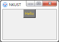 欲讓按鈕按下執行某些指令,僅須在此處設定command參數,讓其值等於某函數(注意只有函數名稱,沒有小括號)即可。不是所有元件都有command參數,僅有例如Button、Checkbutton、與Radiobutton等特定元件有此參數。
現在點擊按鈕確實會印出Hello, World!字樣,而且按一下印一次,不過似乎應該顯示在視窗上感覺比較對,所以再將其修改如下:
def sayHello(): txt.insert(tk.END,"Hello, World!") bt_hello = tk.Button(root,text="Hello", bg='gray', fg='gold', relief='raised', command=sayHello) bt_hello.pack(side=tk.TOP) txt = tk.Text(root, width=50, height=10, bg='lightgreen') txt.pack()
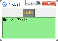 要想將文字顯示在視窗,可以使用之前學過的標籤,這裡使用另一個文字顯示元件text。很簡單就是使用跟其他元件一樣的方法建立一個Text物件然後放置在Button之後,只是在函數sayHello()中改為使用insert()方法將文字加入到txt中,其中第一個參數tk.END表示自最後空白處加入,也就是第一行第一個字,也可以使用
txt.insert('1.0',"Hello, World!")表示自1.0的位置加入。
設定command參數可以呼叫函數,不過這樣的方式好像無法呼叫有輸入參數的函數(因為我們只能給函數名,不能加上小括號,所以無法給輸入值),如果要呼叫有輸入值的函數,我們可以這麼做:
def sayHello(x): txt.insert(tk.END,x) bt_hello = tk.Button(root,text="Hello", bg='gray', fg='gold', relief='raised', command=lambda: sayHello("Hi, there.")) bt_hello.pack(side=tk.TOP) txt = tk.Text(root, width=50, height=10, bg='lightgreen') txt.pack()
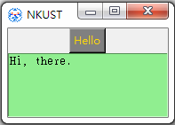 簡單吧!只要使用lambda呼叫該函數,變成傳回一個沒有參數的函數即可。
現在來練習設計一個計算BMI的程式,設計BMI對你來說沒有難度,不過要設計個讓使用者輸入數值的地方,我們可以使用Entry元件,做法如下:
lbWeight = tk.Label(root, text='請輸入體重(kg)') enWeight = tk.Entry(root, width=20) lbHeight = tk.Label(root, text='請輸入身高(m)') enHeight = tk.Entry(root, width=20) btBmi = tk.Button(root, text="BMI", command=Bmi) lbBmi = tk.Label(root)此處設計六個元件,lbWeight與lbHeight是提示用的標籤,而enWeight與enHeight則是讓使用者輸入身高體重的輸入欄,除了設定寬度,還可以比照之前提過的方式設定參數來改變外觀。而btBmi是按鈕,當點擊後會呼叫Bmi()方法。最後此處改使用標籤(lbBmi)來顯示結果。接著可以將這六個元件置入主視窗,直接由上往下排列,所以加上:
lbWeight.pack() enWeight.pack() lbHeight.pack() enHeight.pack() btBmi.pack() lbBmi.pack()最後加上Bmi()方法如下:
def Bmi(): w = float(enWeight.get()) h = float(enHeight.get()) bmi = w/h/h if bmi < 18.5: bmitext="太輕了,要多吃一點" textcolor='green' elif 18.5 <= bmi < 23.9: bmitext="標準身材,請好好保持" textcolor='blue' elif 23.9 <= bmi < 27.9: bmitext="喔喔!得控制一下飲食了,請加油" textcolor='orange' else: bmitext="肥胖容易引起疾病,請注意健康" textcolor='red' lbBmi.config(text=f'BMI={bmi}\n{bmitext}', foreground=textcolor)
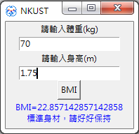 使用get()方法取得Entry內的文字,因為需要的是數字,所以將其cast成為實數。計算bmi各位應該熟極而流,要將文字顯示在標籤內,直接使用config(text)來設定即可,此處也同時讓不同等級的bmi顯示不同顏色的文字。
請試試看設計一個轉換華氏攝氏溫度的視窗程式。
事實上除了使用command之外,我們還需要其他類型的事件回應,例如按下某鍵盤按鍵、滑鼠雙擊、滑鼠右鍵、游標移過某元件等,回應這些事件我們須在元件上讓函數與事件綁定,此時使用bind()方法,舉例如下,設計一個視窗,其中僅包含一個標籤,然後讓不同的事件在標籤上顯示不同的文字。
def toEnter(event): lbShow.config(text="Cursor Enter Widget") def toDouble(event): lbShow.config(text="Double Click.") def toPressKey(event): lbShow.config(text=event.keysym) def toA(event): lbShow.config(text="A is pressed.") def toShift(event): lbShow.config(text="Shift+Up") def toReturn(event): lbShow.config(text="You pressed Return") def toConfigure(event): lbShow.config(text=f"{root.winfo_width()},{root.winfo_height()}") lbShow = tk.Label(root, width=50, height=5, bg='tomato') lbShow.bind("<Enter>",toEnter) lbShow.bind("<Double-Button>",toDouble) root.bind("<a>",toA) root.bind("<Key>",toPressKey) root.bind("<Shift-Up>",toShift) root.bind("<Return>",toReturn) root.bind("<Configure>",toConfigure) lbShow.pack()此處定義數個函數來對應不同的事件,當元件與事件綁定後,便可以執行對應函數,例如lbShow.bind("
事實上跟鍵盤有關的事件多跟視窗綁定,我們可偵測大多數的鍵盤活動,此例中的
所有事件的對應列表請見此話後附表格,也請自行練習相關事件操作。此處再舉一個例子如下,一樣僅設計一個標籤,此標籤綁定兩個事件(
import datetime count=0 start=0 def toEnter(event): global count global start if count==0: start=datetime.datetime.now() count+=1 lbShow.config(text=f"Clicked {count} times", fg="white") def toDouble(event): global count global start end = datetime.datetime.now() period=(end-start).seconds txt = f"You clicked {count} times in {period} seconds." txt += "\nClick Here to restart" lbShow.config(text=txt) count = 0 lbShow = tk.Label(root, text="Click Here to start",width=30, height=5, bg='tomato') lbShow.bind("<Button-1>",toEnter) lbShow.bind("<Button-3>",toDouble) lbShow.pack()
-
Talk123_1.py
- 在Button元件中設定參數command來呼叫函數,若該函數需要輸入值,使用lambda
- 使用bind()方法讓元件與事件結合來執行函數
Recap
| Events | |
|---|---|
| <ButtonRelease> | 放開滑鼠按鍵。<ButtonRelease-1>, <ButtonRelease-2>, <ButtonRelease-3>分別代表放開左中右鍵。可取得滑鼠游標位置。 |
| <Double-Button> | 連按兩次。<Double-Button-1>, <Double-Button-2>, <Double-Button-3>代表連按左中右鍵。 |
| <Enter> | 滑鼠指標進入元件(widget)。(不是按下Enter) |
| <Leave> | 滑鼠指標離開元件(widget)。 |
| <FocusIn> | 鍵盤焦點移至元件(使用tab切換) |
| <FocusOut> | 鍵盤焦點移開元件(使用tab切換) |
| <Return> | 按下Enter鍵。也可使用其他鍵,例如:Cancel(Break), BackSpace, Tab, Return(Enter), Shift_L, Contro_L, Alt_L, Pause, Caps_Lock, Escape, Prior(Page Up), Next(Page Down), End, Home, Left, Up, Right, Down, Print, Insert, Delete, F1~F12, Num_Lock, Scroll_Lock. |
| <Key> | 按下任一鍵。 |
| a | 按下某一鍵,原則上大部分可印出的鍵都可以,除了空白鍵。 |
| <Shift-Up> | 同時按下Shift+Up鍵。也可以跟Alt或Control連用。或是Shift、Alt、Control與滑鼠連用,例如<Control-Button-1>、<Shift-Button-1>、<Control-Shift-Button-1>等。 |
| <Configure> | 元件的大小改變。 |
| <Motion> | 滑鼠移動。<B1-Motion>, <B2-Motion>, <B3-Motion>分別代表按著左中右鍵移動。可取得滑鼠游標位置。 |
第一百二十四話、視窗程式Tkinter之Layout Management
之前提過可以使用pack()來配置視窗元件,如果只是很簡單的幾個元件,好像還可以,不過若是稍微複雜一些,光是使用pack()並不夠好使,靈活度不夠,所以以下介紹其他三招來協助我們配置元件。- Pack()+frame 在之前介紹的widget中,有幾個元件是用來當作容器使用的,例如Frame或是LabelFrame,我們可以將元件放入Frame,再使用pack()來安排Frame的位置,如此便可以調整元件的位置,也就是好比先將文具放鉛筆盒內,再來排列鉛筆盒位置,有道理吧。舉例如下:
import tkinter as tk import tkinter.ttk as ttk root=tk.Tk() root.tk.call('wm','iconphoto',root._w, tk.PhotoImage(file='pics/icon.png')) root.wm_title("NKUST") root.geometry("180x100") root.config(background='#888') fTop = tk.Frame(root, bg="lightblue") fBottom = tk.Frame(root, bg="lightgreen") fLeft = tk.Frame(root, bg="gold") fRight = tk.Frame(root, bg="tomato") fCenter=tk.Frame(root, bg='olive') btTop1 = tk.Button(fTop, text='Button 1') btTop2 = tk.Button(fTop, text='Button 2') btBottom1 = tk.Button(fBottom, text='Button 1') btBottom2 = tk.Button(fBottom, text='Button 2') lbLeft1 = tk.Label(fLeft, text='Label 1', bg='green') lbLeft2 = tk.Label(fLeft, text='Label 2', bg='blue') lbRight1 = tk.Label(fRight, text='Label 1', bg='green') lbRight2 = tk.Label(fRight, text='Label 2', bg='blue') fTop.pack(side=tk.TOP, fill=None) fBottom.pack(side=tk.BOTTOM, fill='x') fLeft.pack(side=tk.LEFT, fill='y') fRight.pack(side=tk.RIGHT, fill='y') fCenter.pack(fill='both',expand=True) btTop1.pack(side=tk.LEFT) btTop2.pack(side=tk.LEFT) btBottom1.pack(side=tk.LEFT) btBottom2.pack(side=tk.LEFT) lbLeft1.pack() lbLeft2.pack() lbRight1.pack() lbRight2.pack() root.mainloop()
 此處程式碼看起來頗長,不過涵義並不多,首先設計五個frame為了放置在上下左右中位置,然後定義四個按鈕(上下各二),四個標籤(左右各二),定義按鈕與標籤時要使用第一個參數註明要被放置在哪個frame內。最後將每個元件都pack()起來擊可,frame顯然有特定方位,正中央的frame只要設定fill='both',expand=True即可延伸。此處特別設定fTop.pack(side=tk.TOP)但是沒有fill,如此因為frame沒有延伸,所以位於正中間。
- place() place()的做法比較直覺,就是將元件放置在特定的座標位置。以下舉例說明,此例中使用與上例相同之元件:
fTop = tk.Frame(root, bg="lightblue", bd=10, relief='raised') fBottom = tk.Frame(root, bg="lightgreen") fLeft = tk.Frame(root, bg="gold") fRight = tk.Frame(root, bg="tomato", width=50) btTop1 = tk.Button(fTop, text='Button 1') btTop2 = tk.Button(fTop, text='Button 2') btBottom1 = tk.Button(fBottom, text='Button 1') btBottom2 = tk.Button(fBottom, text='Button 2') lbLeft1 = tk.Label(fLeft, text='Label 1', bg='green') lbLeft2 = tk.Label(fLeft, text='Label 2', bg='blue') lbRight1 = tk.Label(fRight, text='Label 1', bg='green') lbRight2 = tk.Label(fRight, text='Label 2', bg='blue') fTop.place(x=50, y=0,relx=None, rely=None, relheight=None, relwidth=1.0, width=200) fBottom.pack(side=tk.BOTTOM, fill='x') fLeft.pack(side=tk.LEFT, fill='y') fRight.pack(side=tk.RIGHT, fill='y') btTop1.pack(side=tk.LEFT) btTop2.pack(side=tk.LEFT) btBottom1.pack(side=tk.LEFT) btBottom2.pack(side=tk.LEFT) lbLeft1.pack() lbLeft2.pack() lbRight1.place(in_=fRight,x=0,y=0) lbRight2.place(in_=fRight,x=0,y=50)
 此處的fLeft、fRight、與fBottom三個frame依然是使用pack加入,而fTop則使用place()來加入。place()中的參數x與y必須給值,如此才能將元件的左上角座標對其此座標,通常還可以給寬高數值(width、height)。雖然此例中有給width=200,不過如果你改變視窗大小,會發現寬度其實都是跟視窗等寬,那是因為設定了relwidth=1.0,這個參數的意思是元件的寬度為視窗寬度的relwidth(0~1)倍,顧名思義,relheight就是相對的高度。而relx與rely也是相對x、y的意思,若是給0~1之間的值,放置位置就會跟視窗大小相關。如果設定x=0、y=0會怎樣?你將會發現此元件被壓在fLeft下方。
每個frame內的元件都是使用pack()置入,除了fRight內的標籤,此兩標籤lbRight1與lbRight2是使用place()方法置入,為了強調是放入fRight這個容器內,所以特別標明in_參數為fRight,之後的x、y座標則是對應fRight的位置了。此處沒有加上中間的fCenter,因為很難控制此區域的大小,若是使用pack(expand=True)將會覆蓋其他元件,若是設定固定大小或是相對大小,在縮放視窗時也會跟其他元件衝突,所以並不好使。 - grid grid()的概念是將原視窗切分為幾個行列(row and column),然後將元件放在特定位置的行列格內,舉例如下:
root.columnconfigure(1, weight=1) root.rowconfigure(1, weight=1) fTop = tk.Frame(root, bg="lightblue") fBottom = tk.Frame(root, bg="lightgreen") fLeft = tk.Frame(root, bg="gold") fRight = tk.Frame(root, bg="tomato") fCenter=tk.Frame(root, bg='red') btTop1 = tk.Button(fTop, text='Button 1') btTop2 = tk.Button(fTop, text='Button 2') btBottom1 = tk.Button(fBottom, text='Button 1') btBottom2 = tk.Button(fBottom, text='Button 2') lbLeft1 = tk.Label(fLeft, text='Label 1', bg='green') lbLeft2 = tk.Label(fLeft, text='Label 2', bg='blue') lbRight1 = tk.Label(fRight, text='Label 1', bg='green') lbRight2 = tk.Label(fRight, text='Label 2', bg='blue') lbCenter=tk.Label(fCenter, text="Center Label",bg='pink') fTop.grid(row=0, column=1, stick='n') fCenter.grid(row=1,column=1, stick='NEWS') fBottom.grid(row=2, column=0, columnspan=3, stick='NEWS') fLeft.grid(row=1,column=0, stick='NEWS') fRight.grid(row=1, column=2, stick='NEWS') fBottom.grid(row=2, column=0, columnspan=3, stick='NEWS') btTop1.pack(side=tk.LEFT) btTop2.pack(side=tk.LEFT) btBottom1.grid(row=0,column=0,padx=10) btBottom2.grid(row=0, column=1) lbLeft1.grid(row=0,column=0) lbLeft2.grid(row=1,column=0) lbRight1.pack() lbRight2.pack() lbCenter.pack(fill='both',expand=True)
 此例依然借用前例的元件,為了讓中間Frame有包含元件,額外設計了lbCenter標籤用來放置於fCenter內。Grid()方法最主要要給值的參數便是row跟column,此兩參數表明該元件被置放的網格位置,自左上角由0開始計數。Stick參數跟之前類似,表示元件的對齊方位,而給NEWS表示元件向四方擴展,若是要表示左右擴展則給WE,若是要表示上下擴展則給值NS。而columnspan與rowspan表示該元件會跨越幾個欄或幾行。若是想要讓元件之間有空隙,跟之前一樣可以設定padx與pady參數。
此時觀察結果會發現雖然配置形狀出來了,但是卻不跟視窗大小連動,所以我們還需要設定root.columnconfigure(1, weight=1) root.rowconfigure(1, weight=1)
所謂的columnconfigure()與rowconfigure()是用來設定行與欄,第一個參數表示編號為1的欄(或行),而weight的值等於1表示第一個參數對應的欄或行會隨著視窗大小而縮放,因為兩者第一個參數皆為1,表示第一行第一欄(也就是正中間的fCenter)會跟著視窗大小連動。
-
Talk124_1.py
- 使用Pack()+frame、place()、grid()等方法可以配置元件。彼此之間或可搭配使用,但較難與place()搭配,可利用frame來群組元件
Recap
第一百二十五話、視窗程式Tkinter之老生常談(I)
接下來舉個例子練習,預定的題目是根據給定的點,找到一個旅行推銷員問題路徑(意思就是一個路線經過平面上特定的點一次且僅有一次,並形成一個頭尾相連的路線,或說是最後回到原出發點),我們的目標是建立一個視窗程式,可以根據給定之題目來找出路徑並繪圖表示。首先要建立視窗架構,先做基本設定如下:
def main(): root=tk.Tk() img = ImageTk.PhotoImage(Image.open("pics/icon.png")) root.tk.call('wm','iconphoto',root._w, img) root.wm_title("NKUST") root.geometry("1000x800") root.config(background='#888') App(root) root.mainloop() if __name__=="__main__": main()此處建立一個函數main()來包含所有設定,這樣可以方便我們整理程式碼,當然一定要導入相關模組,如下:
import tkinter as tk from tkinter import ttk from PIL import Image, ImageTk在main()中有一個陌生的指令是App(root),表示我們欲設計一個物件稱之為App,並讓root作為初始參數。這個App物件會總管整個視窗的配置,程式碼如下:
class App(): def __init__(self, root): self.root = root container = tk.Frame(self.root) container.pack(side=tk.TOP, fill=tk.BOTH, expand=True) container.grid_rowconfigure(1, weight=1) container.grid_columnconfigure(0, weight=1) iconbar = IconBar(container, self) iconbar.grid(row=0, column=0, sticky="n") self.frames = {} for F in (PageOne, PageTwo, PageThree): frame = F(container, self) self.frames[F] = frame frame.grid(row=1, column=0, sticky="nsew") self.showFrame(PageOne) def showFrame(self, cont): frame = self.frames[cont] frame.tkraise()解釋一下,首先是__init__()方法,傳入root作為參數,並讓其等於self.root變數。接著是設計一個名為container的frame,這個container是一個大容器,pack的時候fill=tk.BOTH且expand=True,表示範圍是整個視窗,我們讓其他的元件在這個大容器中配置。
而要配置在這個container內的元件,主要分為兩個,第一個是iconbar,第二個是frames。使用grid()來配置這兩個元件,menubar放在row=0, column=0,而frames放在row=1, column=0的位置,表示一上一下。
而
container.grid_rowconfigure(1, weight=1)與
container.grid_columnconfigure(0, weight=1)這兩行指令是grid的設定,表示當視窗改變大小的時候,row=1、columns=0的元件會跟著視窗縮放。weight=1表示會縮放,等於0表示不會。
可以看到frames是一個dict,其實其中包含不只一個frame,在此設計三個,此三個frame的放置位置都相同(row=1, column=0),表示三個疊在一起,那麼會顯示哪一個?在此設計另一個方法稱為showFrame(),只要傳入某frame,使用tkraise()方法讓該frame浮現。
由上可知iconbar是IconBar物件,先看IconBar物件的設計:
class IconBar(tk.Frame): def __init__(self, parent, controller): tk.Frame.__init__(self,parent, bg='blue') button1 = ttk.Button(self, text="Visit Page 1", command=lambda: controller.showFrame(PageOne)) button1.pack(side=tk.LEFT) button2 = ttk.Button(self, text="Visit Page 2", command=lambda: controller.showFrame(PageTwo)) button2.pack(side="left") button3 = ttk.Button(self, text="Visit Page 3", command=lambda: controller.showFrame(PageThree)) button3.pack(side="left")IconBar物件繼承自tk.Frame,這當然使得它本身是個frame,而在初始化方法(__init__)中,我們設計它須傳入兩個參數,parent與controller。parent是父容器,也就是這個元件要被放置的容器,使用tk.Frame.__init__(self, parent)方法來定義,表示這個frame要放置的容器是parent。同時也可以在此設定參數,所以加上一個bg='blue',你也可以加上其他參數設定。
在此IconBar中加入三個button,分別對應三個頁面的frame。設置方法你應該沒有問題,此處加上command讓按鈕按下後呼叫showFrame()方法,此方法因為有輸入值,所以使用lambda,因為此方法是屬於App內的方法,所以使用controller替代,也就是說如果要宣告IconBar時,需要傳入此IconBar的父容器以及一個可以呼叫showFrame()方法的物件,也就是App物件。這也說明了在App中的這行指令iconbar = IconBar (container, self),建立名為iconbar的IconBar物件,此iconbar將放置在container內,第二個參數self指的便是App本身。
而frames內包含的三個frame,分別是屬於PageOne、PageTwo、PageThree三個物件,因為三者的初始型態相同,所以直接使用一個for loop來一併宣告,frame = F(container, self)跟Menu的宣告其實相同,一個父容器,一個App本身,我們來看這三個物件的設計:
class PageOne(tk.Frame): def __init__(self, parent, controller): tk.Frame.__init__(self, parent, bg='red') label = tk.Label(self, text="This is the page one") label.pack(pady=10, padx=10) class PageTwo(tk.Frame): def __init__(self, parent, controller): tk.Frame.__init__(self, parent, bg='green') label = tk.Label(self, text="This is the page two") label.pack(pady=10, padx=10) class PageThree(tk.Frame): def __init__(self, parent, controller): tk.Frame.__init__(self,parent, bg='orange') label = ttk.Label(self, text="Page Three", font=Font1) label.pack(pady=10,padx=10)因為之後要在各自頁面加上不同的內容,所以在此每一個頁面設計一個對應的class。一開始沒有內容,所以隨便加個label顯示文字意思一下。在PageThree中有個font=Font1,事實上只是在程式碼上端設計的一個全域變數Font1 = ("Verdana", 12),我們可以利用這樣的方式設計幾個喜歡的型態,然後在想要改變文字顯示方式的地方直接給font參數數值,可以較容易管理。 總結一下,這個視窗架構內含一個主要的frame稱為container,container內包含兩部分,上部是iconbar,屬於IconBar物件的frame,下部是三個frame疊在一起,分別是PageOne、PageTwo、PageThree,合成一個frames的list。iconbar內的有三個按鈕,分別對應三個頁面,按下去後便會浮現對應的頁面。顯示結果如下圖:
第一百二十六話、視窗程式Tkinter之老生常談(II)
接下來我們開始修改個別頁面的內容,首先看PageOne。在PageOne類別中定義了數個函數,先看第一個初始化函數:class PageOne(tk.Frame): def __init__(self, parent, controller): tk.Frame.__init__(self, parent, bg='azure') self.lbNode = tk.Label(self, text="Number of Nodes:") self.lbNode.grid(row=0, column=0, padx=20, pady=10) self.enNode = tk.Entry(self) self.enNode.grid(row=0, column=1) self.lbSeed = tk.Label(self, text="Seed:") self.lbSeed.grid(row=1, column=0, padx=20, pady=10) self.enSeed = tk.Entry(self) self.enSeed.grid(row=1, column=1) self.btRun = tk.Button(self, text="Run") self.btRun.grid(row=2, column=0, columnspan=2, padx=20, pady=10) self.btRun.bind("<Button-1>", self.route) self.txtResult = tk.Text(self, bg='deepskyblue', width=100, height=20) self.txtResult.grid(row=3, column=0, columnspan=2, padx=20, pady=10)PageOne的配置如上,其中設置了兩個標籤(lbNode、lbSeed)顯示提示文字,兩個Entry(enNode、enSeed)分別用來輸入數值節點個數與隨機種子,一個按鈕(btRun)用來執行函數,再加上一個Text(txtResult)用來顯示結果。這些元件都使用grid()來配置版面位置。此處按鈕與函數使用bind()方法連結,對應的事件函數為route(),內容如下:
def route(self, event): nnodes = int(self.enNode.get()) seed = int(self.enSeed.get()) appText = f"Number of nodes={nnodes}\t seed={seed}" global nodes nodes = pd.DataFrame(np.arange(nnodes), columns=["ID"]) np.random.seed(seed) nodes['x'] = np.random.randint(1,100,nnodes) nodes['y'] = np.random.randint(1,100,nnodes) np.random.seed() shortestDis = self.shortest(10) r = [i for i in nodes['ID']] appText += f"\nroute: {str(r)}\nTotal Distance={shortestDis}\n\n" #print(nodes) self.txtResult.insert(tk.END, chars=appText)此函數根據所輸入的點數與亂數種子產生題目,並呼叫shortest()方法計算路徑長度。為了讓其他方法也能取得nodes這個DataFrame的資料,所以將其定義在最前面nodes=None,然後在方法中使用global nodes來取得它。那麼shortest()這個方法的內容呢?
def shortest(self, times): global nodes dis = self.routeLength() for i in range(times): nodes['ran'] = np.random.rand(len(nodes)) nodes.sort_values(by='ran', inplace=True) newDis = self.routeLength() if newDis < dis: dis = newDis return dis求得路徑的方式只是很簡單的將順序打亂(shuffle),在此做法是在nodes內加上一個名為ran的欄,隨機產生亂數填滿,然後根據此欄的值排序,排序的時候設定inplace=True,直接修改nodes內的順序。為了得到較好的解,這個方法設定輸入參數times,如此可以執行多次來找到較好的路線。根據前面的呼叫方法,設定的times為10,如果你願意的話也可以設計一個Entry來讓使用者輸入執行次數。
而求得一解的路線長度方法是routeLength(),內容如下:
def routeLength(self): global nodes r = [i for i in nodes['ID']] totalDis = 0 for i in range(len(r)-1): totalDis += self.length(nodes.loc[r[i]]['x'], nodes.loc[r[i]]['y'], nodes.loc[r[i+1]]['x'], nodes.loc[r[i+1]]['y']) totalDis += self.length(nodes.loc[r[0]]['x'], nodes.loc[r[0]]['y'], nodes.loc[r[-1]]['x'], nodes.loc[r[-1]]['y']) return totalDis這倒是沒甚麼,只是取得利用洗牌過後的ID,依序逐點計算距離然後相加,因為是頭尾相接的路線(也就是會回到出發點),所以要記得再加上頭尾的距離。計算兩點間距離的方法length()就沒啥好說的了,如下:
def length(self, x1, y1, x2, y2): return ((x1-x2)**2+(y1-y2)**2)**0.5執行程式後顯示結果如下:

第一百二十七話、視窗程式Tkinter之老生常談(III)
在有了數值之後,我們想要使用Matplotlib繪製適才求得的解,然後顯示在PageTwo內,這裡主要的做法是寫成一個方法在PageTwo物件內,如下:def showFigure(self): f = Figure(figsize=(5,5), dpi=100) ax = f.add_subplot(111) x = list(nodes['x']) x.append(nodes['x'].iloc[0]) y = list(nodes['y']) y.append(nodes['y'].iloc[0]) ax.plot(x, y, marker='D', markersize=5, color='b', mec='r', mfc='g') #建立畫布並將圖繪入 canvas=FigureCanvasTkAgg(f, master=self) canvas.draw() canvas.get_tk_widget().pack(side=tk.TOP, fill=tk.BOTH, expand=True) #顯示工具列 toolbar = NavigationToolbar2Tk(canvas,self) toolbar.update() canvas._tkcanvas.pack(side=tk.TOP, fill=tk.BOTH, expand=True)將matpltlib的圖在tkinter中顯示的步驟主要有三部曲,在使用之前我們需要先導入所需要的模組,如下:
from matplotlib.backends.backend_tkagg import FigureCanvasTkAgg, NavigationToolbar2Tk from matplotlib.figure import Figure第一部曲是繪製圖案,為了將圖繪入canvas然後嵌入視窗顯示,首先建立一個Figure,然後在其中加入subplot,因為只放一圖,所以參數是111,你應該還記得。然後使用傳回的軸物件ax呼叫plot()繪圖(使用matplotlib繪圖,所以也可以使用例如bar()來繪製,端看你需要的顯示方式)。其中的x、y因為要多繪製頭尾相連的線段,所以經過一番整理,你應該可以讀懂。
第二部曲有三個步驟,使用FigureCanvasTkAgg()建立畫布,使用canvas.draw()在畫布上繪圖,然後將畫布pack()。
而第三部曲也是三步驟,這一個部分是為了要加入工具列,可做可不做,不過當然有內建工具列比較好,方便我們觀察或操作。首先使用NavigationToolbar2Tk()建立toolbar,然後使用update()更新,接下來一樣pack()即可。
因為要等nodes有內容才能繪圖,不然會出現Nonetype錯誤,所以我們在PageTwo的初始化方法內再設計一個按鈕,此按鈕按下去才會開始繪圖,如下:
class PageTwo(tk.Frame): def __init__(self, parent, controller): tk.Frame.__init__(self, parent, bg='green') btShow = tk.Button(self, text='Show', command=self.showFigure) btShow.pack()執行程式後,先在第一頁輸入數值然後計算,接下來再到第二頁點擊按鈕來顯示圖形,結果顯示如下:
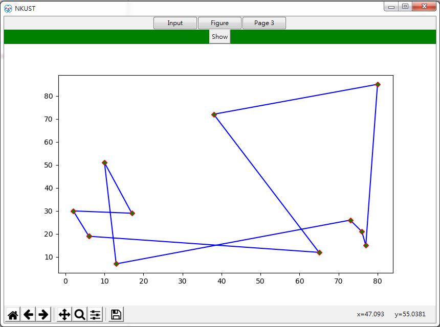
第一百二十八話、視窗程式Tkinter之老生常談(IV)
現在我們假設有一個穩定的訊號源,我們想寫程式持續去取得這些資料然後繪圖。舉例來說在某些網站可能會持續的更新例如股票的漲跌資料,或是某路段的交通速度資料,也許幾分鐘就會更新一次,若是我們可以寫程式持續地取得這些資料來分析處理繪圖,便是一個動態的分析結果。要達到這樣的效果,首先寫一個小程式來模擬這樣的信號源,做法如下Talk128_2.py:import time import numpy as np from datetime import datetime as dt def gen(): return np.random.randint(70,100) while True: time.sleep(30) with open('talk128_2.txt','a') as f: f.write(f"{dt.now().strftime('%H-%M-%S')},{gen()},{gen()}\n")這個簡單程式利用time.sleep()方法,每30秒啟動一次,然後將時間與兩個數據寫入到Talk128_2.txt這個檔案內。完成之後在Spyder上方工具列選擇Console>Open an IPython console,點選之後出現一個新的console(Console 2/A),讓程式在此console執行,便會持續更新檔案,只是沒有設計停止機制,只能使用Ctrl+c強制中止(或是在console的右上方會有一個正方形,顯示紅色,點即以停止),或是將while loop改為for loop,讓其僅產生特定數量的資料。
再來我們就可以持續定時讀取此檔案中資料,然後繪製內容並顯示在Page3。將PageThree()修改如下:
class PageThree(tk.Frame): def __init__(self, parent, controller): tk.Frame.__init__(self,parent, bg='orange') #建立畫布並將圖繪入 canvas=FigureCanvasTkAgg(f3, master=self) canvas.draw() canvas.get_tk_widget().pack(side=tk.TOP, fill=tk.BOTH, expand=True) #顯示工具列 toolbar = NavigationToolbar2Tk(canvas,self) toolbar.update() canvas._tkcanvas.pack(side=tk.TOP, fill=tk.BOTH, expand=True)此處跟之前秀圖的做法類似,保留後面兩步驟,在FigureCanvasTkAgg(f3)裡面使用f3這個figure,是我們接下來要建立的figure。這個class會在程式開始執行時便開示將f3顯示在Page3頁面。接著在class外層加上以下程式碼:
f3 = Figure(figsize=(5,5), dpi=100) ax3 = f3.add_subplot(111)如此便跟前一話所提的三部曲相同了,現在只要繪圖即可。因為我們需要定時的取得資料並繪製,所以要將繪圖的步驟寫成一個函數,然後定時的呼叫它,又因為剛才我們建立的訊號源將利用時間做為x軸,因為我們需要導入以下模組:
from matplotlib import animation from datetime import datetime as dt import matplotlib.dates as mdates其中datetime與dates之前都介紹過,而animation可以幫助我們定時呼叫函數,函數的寫法如下:
def animate(i): pullData=None with open('talk128_2.txt','r') as f: pullData =f.read() dataArray = pullData.split('\n') x = [] y1 = [] y2 = [] for eachLine in dataArray: if len(eachLine)>1: xx, yy1, yy2 = eachLine.split(',') x.append(dt.strptime(xx, "%H-%M-%S")) y1.append(int(yy1)) y2.append(int(yy2)) ax3.clear() ax3.set_title(f"Reality vs. Prediction\nLast:{y1[-1]}:{y2[-1]}") ax3.plot(x,y1, 'b-', x, y2, 'r:') #plot timeFmt = mdates.DateFormatter("%H-%M") minutes = mdates.MinuteLocator(interval=10) ax3.xaxis.set_major_locator(minutes) ax3.xaxis.set_major_formatter(timeFmt) ax3.legend(bbox_to_anchor=(0,0.98,1,.1), loc=0, labels=('Reality','Prediction'), ncol=2)這個函數首先開啟連結到檔案,然後讀取所有資料並儲存在pullData變數。使用split('\n')來將資料拆成一行一行的加入dataArray這個list,然後針對每一行再使用split(',')來切分為三個資訊值,姑且稱為時間、真實值、預測值,分別儲存在list內。時間的部分使用strptime()來將字串轉匯成時間物件,並在每次繪圖錢加上ax3.clear()來清除舊圖,然後便可以繪製了。
剩下的主要是控制x軸的顯示,因為訊號源每30秒更新一次,在x軸使用locator()控制每10分鐘一個tick label。最後到main()加上
ani = animation.FuncAnimation(f3, animate, interval=30000) root.mainloop()讓函數animate()每30秒啟動一次,這行顯然需要寫在mainloop()之前,不然視窗都關閉了。現在可以執行程式看看結果如何,直接點擊page3應可看到繪製的圖。
接下來還能做一點美工,例如前面學過的加上以下:
from matplotlib import style style.use('bmh')或是讓程式視窗出現時坐落在螢幕正中間,如下:
def main(): root=tk.Tk() img = ImageTk.PhotoImage(Image.open("pics/icon.png")) root.tk.call('wm','iconphoto',root._w, img) root.wm_title("NKUST") screenwidth = root.winfo_screenwidth() screenheight = root.winfo_screenheight() w = 1280 h = 800 tox = int((screenwidth-w)/2) toy = int((screenheight-h)/2) size = f"{w}x{h}+{tox}+{toy}" root.geometry(size) root.config(background='#888') App(root) ani = animation.FuncAnimation(f3, animate, interval=1000) root.mainloop()winfo_screenwidth()與winfo_screenheight()兩方法可以取得螢幕寬度與高度。再者因為後續內容會越來越多,圖會越畫越寬,若是僅需要最後的幾筆,可以在函數animate()內將plot()改行使用以下程式碼代替。
設定showrange為50,那麼便可持續顯示最後的50筆資料。最後圖形顯示如下:

第一百二十九話、視窗程式Tkinter之老生常談(V)
在視窗上方安排的按鈕類似快捷鍵,接著我們預計在其上再加上下拉式選單。做法也容易,在App()的__init__()內加上以下程式碼:mbar = tk.Menu(container) filemenu = tk.Menu(mbar, tearoff=0) filemenu.add_command(label="Save", command = self.save) filemenu.add_separator() filemenu.add_command(label="Exit", command=self.root.destroy) mbar.add_cascade(label="File", menu=filemenu) self.root.config(menu=mbar)首先使用tk.Menu()建立一個menubar,參數是container,意思就是在container視窗上方建立一個選項,在之後我們使用add_cascade()方法定義此選項的顯示名稱以及內含選單,此方法的參數為label= "File",表示會出現File字樣,然後另一個參數是menu=filemenu,表示在這個選項的內含選單,也就是中間部分建立的filemenu,到最後再使用config讓這個mbar掛上選單列。聽起來很拗口,到處都是menu,看一下圖體會一下:
 這樣就清晰很多了,一個選項File,其下有一選單,兩個選項分別是Save與Exit。這個下拉選單的做法就是再使用tk.Menu()方法,不過其中有個tearoff參數,這裡設定是0(或使用False),所以沒看到甚麼,若是設定為1(或True),就會出現一條虛線,點擊後這個下拉選單會變成單獨的視窗,就這樣。在Save與Exit之間有一條線,很明顯是因為加上add_seperator()這個方法產生的。而最重要的選項Save與Exit是使用add_command()方法建立,顯示名稱使用label參數設定,跟按鈕一樣,使用command來呼叫函數,讓點擊有反應。函數save馬上介紹,至於self.root.destroy這個方法會中斷mainloop()來結束視窗程式。
來看看save這個方法,其實我們這裡也沒甚麼要儲存的,假設要儲存顯示在Page3的資料好了,簡單的方式可以這樣做:
def save(self): with open('save129.txt', 'a') as f: with open('talk128_2.txt', 'r') as f2: da = f2.read().split('\n') if len(da) < showrange: for i in da: f.write(f"{i}\n") else: for i in range(-showrange, -1): f.write(f"{da[i]}\n") tk.messagebox.showinfo("Info", "File Saved.")這對我們來說沒甚麼,開啟兩個檔案連結,一個讀一個寫,只是這裏我們只要後面特定數量的資料。最後一行的messagebox倒是沒甚麼,會跳出來一個視窗顯示存檔完成,可做可不做,有的好處只是確認一下存檔完成。
這樣的做法僅能將資料儲存在與程式相同的資料夾,使用filedialog來建立檔案選擇視窗,可以讓我們選擇檔案與路徑,記得要導入from tkinter import filedialog。
def save(self): filename = filedialog.asksaveasfilename( initialdir="/", title="Save as", filetypes=(("text files","*.txt"),("all files","*.*"))) with open(filename, 'a') as f: with open('talk128_2.txt','r') as f2: da = f2.read().split('\n') if len(da) < showrange: for i in da: f.write(f"{i}\n") else: for i in range(-showrange, -1): f.write(f"{da[i]}\n")使用filedialog可以呼叫asksaveasfilename、askopenfilename等,對應不同操作,參數initialdir是一開啟的資料夾路徑,title是此視窗之標題,而filetypes顯然是顯示的檔案類型。有了檔案名稱與路徑其餘就沒有懸念了,因此已經開啟存檔視窗,在此就不再開啟提示資訊視窗。
現在再增加一個選單,通常一個視窗程式常會有個help(一般是按F1)來解釋如何使用之類的,所以現在先加上以下程式碼來建立選單:
helpmenu = tk.Menu(mbar, tearoff=True) helpmenu.add_command(label="Version", command = lambda: tk.messagebox.showinfo(title="Version", message="Version 1.0")) helpmenu.add_separator() helpmenu.add_command(label="Tutorial", command = lambda: self.tutorial("<Button-1>")) mbar.add_cascade(label="Help", menu=helpmenu) self.root.bind("<F1>", self.tutorial) self.root.config(menu=mbar)此處跟之前介紹的做法差不多,值得一提的是self.tutorial()這個方法在兩個地方被提及,第一個是事件為
def tutorial(self, event): mess = "This program is a window-application of Tkinter." tk.messagebox.showinfo(title="Tutorial", message=mess)跟之前的做法一樣,Eazy。因為mess的文字很長,此處不列出,點擊後出現結果如下:
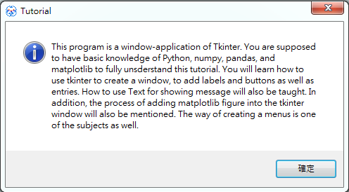 其實也就是再產生一個視窗,所以也可以直接產生新視窗,產生的方法除了tk.Tk()之外,還能夠使用tk.Toplevel(),這裡使用Toplevel()示範:
def tutorial(self, event): t = tk.Toplevel() mess = "This program is a window-application of Tkinter." messText = tk.Label(t, wraplength=300, justify=tk.LEFT, text=mess, background="lightgreen") #messText.insert(tk.END, chars = mess) messText.pack() btOk = tk.Button(t, text="OK", command=t.destroy) btOk.pack() t.mainloop()此處建立一個Label來顯示文字訊息,參數wraplength用來控制每行的最大長度,之後加上一個按鈕用來關閉視窗。顯示結果如下,將Toplevel()換成Tk()效果相同。
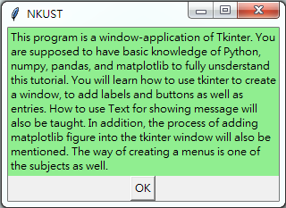 教學或是Help有的時候內容相當多,此時也許需要多頁來顯示,我們當然可以直接建立一個視窗,再使用此範例的類似方法,建立一個IconBar來容納多個icon,並讓它們觸發新頁面的產生。原則上就幾乎是把之前做得再做一次類似的。此處換利用另一個方式,讓我們把內容安排成數頁,並且可以一頁頁往下讀。做法介紹如下,假定我們有三頁的說明內容以及一個首頁,首先在tutorial()內加上
tutStart = tk.Tk() tutStart.geometry("+500+300") btStart = tk.Button(tutStart, text="Start Tutorials", command=Page1) btStart.pack() datamess = "The data is generated randomly use np.random()" btData = tk.Button(tutStart, text="What are the data?", command= lambda: tk.messagebox.showinfo(title="Data", message=datamess)) btData.pack() tutStart.mainloop()這部分是首頁的內容,其中包含兩個按鈕,其中第二個按鈕是示範假定我們想詢問資料來源甚麼的,不見得要有,只是代表我們可以加上一堆按鈕,如果我們有那麼多類型的內容說明的話。第一個按鈕是讓我們開始顯示教學的第一頁,很明顯在tutorial內,有一個方法稱為Page1,以下為Page1內容,必須將此方法加在tutStart=tk.Tk()這行前面,如下:
def Page1(): tutStart.destroy() t1 = tk.Tk() def Page2(): t1.destroy() t2 = tk.Tk() def Page3(): t2.destroy() t3 = tk.Tk()Page1()的架構如上,其中包含了Page2()函數,而Page2()內又包含了Page3(),且每次進入另一頁面,第一件事便是終止前一頁面,然後建立新的視窗頁面,這樣的方式可以讓我們一頁一頁往下讀。而每一頁的內容原則上就是要顯示部分的幫助內容,例如第一頁是:
t1.geometry("+500+300") mess1 = "This program is a window-application of Tkinter." lbText1 = tk.Label(t1, text=mess1, wraplength=300, justify=tk.LEFT, background='lightgreen') lbText1.pack() btNext1 = tk.Button(t1, text="Next", command=Page2) btNext1.pack() t1.mainloop()此處一樣建立一個Label來顯示文字並建立一個按鈕Next來呼叫下一頁,下一頁一開始便會呼叫destroy()來摧毀前一頁。如果有很多頁便如此一路往下寫。最後一頁(在此為Page3),做法則如下:
t3.geometry("+500+300") mess3 = "This program is a window-application of Tkinter." lbText3 = tk.Label(t3, text=mess3, wraplength=300, justify=tk.LEFT, background='lightblue') lbText3.pack() btDone = tk.Button(t3, text="Done", command=t3.destroy) btDone.pack() t3.mainloop()可以看出來沒啥不同,只是按鈕的command變成是關閉視窗。
第一百三十話、視窗程式Tkinter之執行檔
當我們完成了一個程式,如果要在其他電腦中執行,可以直接將檔案傳到該電腦,只要那裏有安裝Python(當然該有的模組都要有安裝)即可執行程式。而若是沒有安裝相關環境的話,此時若是可以將我們設計的程式包裝成一個自執行檔,也就是不需要有相關環境即可執行的檔案,也是可以執行。要做到這一點有好幾個應用程式可以達成(e.g. py2exe、cx_Freeze、PyInstaller等),在此採用PyInstaller,進行步驟如下:首先安裝PyInstaller,在開始工作表找到Anaconda Prompt,跟DOS一樣的,在指令列輸入pip install pyinstaller,然後應該就會開始安裝。
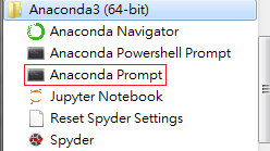
- 安裝完畢後應該就可以開始使用了。首先先練習一下最簡單的,設計一個hello.py,其內只有一行指令print("Hello"),設計一個獨立的資料夾將此檔案放入,其他無關的資料檔案都不需要。在Prompt中使用cd指令到檔案所在之資料夾,然後輸入pyinstaller –F hello.py,
 之後便會開始執行,因為hello.py內容很少,所以應該不用多久就會出現Building EXE from EXE-00.toc completed successfully字樣,表示執行成功。

-
接下來到資料夾中會看到多了一些資料夾,如下:
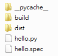 執行檔就在資料夾dist內,你會看到
 雙擊執行。會出現一個DOS視窗,不過應該會抖一下還沒看清楚就關閉了,那是因為執行完畢就關了,若是要讓其保持開啟,可以在程式中加上一行input(),這樣程式會以為有輸入,視窗便不關閉,如下:
print("Hello") input()
接著用檔案總管到對應的資料夾,把剛才產生的內容都刪去(也就是僅留下hello.py),然後到Prompt在執行一次pyinstaller –F hello.py,等完成後,一樣雙擊hello.exe執行程式,結果如下: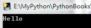
-
接下來試試看tkinter的相關程式,首先一樣設計一個簡單的程式(tkinterexe.py)然後放到一個獨立的資料夾,程式內容如下:
import tkinter as tk root=tk.Tk() root.tk.call('wm','iconphoto',root._w, tk.PhotoImage(file='icon.png')) root.title("NKUST") root.geometry("300x200") lb = tk.Label(root, text="Hello") lb.pack(side='top', fill='x', expand=True) root.mainloop()
應該是最簡單的了,一樣使用Prompt到對應的資料夾,然後輸入 等等,這裡多了一個-w?如果沒有-w當然是OK的,只是執行的時候會有DOS視窗,對於視窗程式並無作用(除非程式需要在DOS內顯示文字(e.g. 使用print())),所以加上-w讓DOS視窗不出現。
執行完後顯示完成,一樣到資料夾dist內找到執行檔(tkinterexe.exe)。不過這個程式需要讀取icon.png這個檔案來顯示視窗icon,所以我們必須將此圖檔複製到此,如下: 接下來雙擊tkinterexe.exe就沒問題了。
img = ImageTk.PhotoImage(Image.open("icon.png")),前一話的例子是將圖放在pics資料夾內,除非我們之後在dist內在建立一個資料夾pics然後才複製圖過去。接著還是一樣執行pyinstaller –F –w Example.py,如果你運氣好,恭喜一次就成功了,若是出現以下的錯誤,
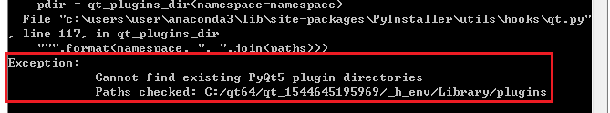 解救方法是先到開始選單的搜尋程式或資料夾(不同版本的Windows可能介面不大相同,原則上就是搜尋全機),輸入PyQt5搜尋,你會找到一個資料夾Library\plugins如下:
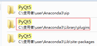 點擊進去裡面有一個檔案(pyqt5qmlplugin.dll)如下:
 接下來建立在提示要檢查的路徑(Paths checked),也就是要建立類似如下的資料夾路徑:
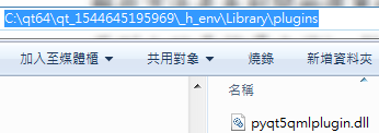 然後將剛才找到的檔案(pyqt5qmlplugin.dll)複製到此新建的資料夾,如上圖。
好累,接下來再回到Prompt再次執行pyinstaller –F –w Example.py(記得先到對應資料夾將上一次執行產生的檔案及資料夾刪除,也就是僅剩下Example.py即可)。因為程式內容牽扯到較多的模組,所以時間也會較長。
執行完成後,再到資料夾dist應可見到Example.exe,幾乎大功告成了,因為此程式會需要呼叫icon圖檔以及文字檔talk128_2.txt,所以需要將相關檔案複製過去,如下:
然後將剛才找到的檔案(pyqt5qmlplugin.dll)複製到此新建的資料夾,如上圖。
好累,接下來再回到Prompt再次執行pyinstaller –F –w Example.py(記得先到對應資料夾將上一次執行產生的檔案及資料夾刪除,也就是僅剩下Example.py即可)。因為程式內容牽扯到較多的模組,所以時間也會較長。
執行完成後,再到資料夾dist應可見到Example.exe,幾乎大功告成了,因為此程式會需要呼叫icon圖檔以及文字檔talk128_2.txt,所以需要將相關檔案複製過去,如下:
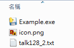 現在雙擊Example.exe應該就可以了,應該需要花個幾秒才會開始執行,要稍稍等待。希望之後Anaconda能夠設計一個按鈕,讓這整個流程一鍵搞定。若對其他建立.exe檔的方法有興趣,只要google就能找到對應做法教學。
Data Structure using Python
Linked List
- Linked List
class Node(object): def __init__(self, sushi, p=None, n=None): self.sushi = sushi self.pre = p self.next = n def __str__(self): return self.sushi __repr__=__str__ class LList(object): def __init__(self, current=None, head=None, tail=None): self.current = current self.head = head self.tail = tail self.size = 0 def insertBefore(self, content): """ * Insert a node containing content in the beginning of the linked list(as the new head) """ if self.head is None: self.head = Node(content) self.tail = self.head else: newNode = Node(content) self.head.pre = newNode newNode.next = self.head self.head = newNode self.size += 1 def insertAfter(self, content): """ * Insert a node containing content at the end of linkedlist(append as the new tail) """ if self.head is None: self.head = Node(content) self.tail = self.head else: newNode = Node(content) self.tail.next = newNode newNode.pre = self.tail self.tail = newNode self.size += 1 def search(self, content): """ * Search the linked list to find the node containing content * Return False if the node is not existed """ if self.head is None: return False else: self.current = self.head for i in range(self.size): if self.current.sushi == content: # print(f"{self.current.sushi} <> {content}") return True else: # print(f"{self.current.sushi} <> {content}") self.current = self.current.next return False def remove(self, content): """ * Delete a node containing content * Return False if the node is not existed """ if self.head is None: return False elif self.head.sushi == content: if self.size==1: self.head = None self.tail = None self.current = None else: self.head = self.head.next self.size -= 1 return True elif self.tail.sushi == content: if self.size==1: self.head = None self.tail = None self.current = None else: self.tail = self.tail.pre self.size -= 1 return True else: self.current = self.head for i in range(self.size): if self.current.sushi == content: self.current.pre.next = self.current.next self.current.next.pre = self.current.pre self.size -= 1 return True else: self.current = self.current.next return False def __iter__(self): """ * To make the linked list iterable """ # return Iterator(self.head) temp = self.head while temp is not None: yield temp temp = temp.next def printLList(self): """ * Print out all the elements inside the linked list """ print("\n==============\n") self.current = self.head for i in range(self.size): print(self.current) self.current = self.current.next def printLList2(self): """ * Print out all the elements inside the linked list """ print("\n============\n") self.current = self.head while self.current is not None: print(self.current) self.current = self.current.next def __str__(self): llstring = "" self.current = self.head while self.current is not None: llstring += f"{self.current} " self.current = self.current.next return llstring __repr__ = __str__ # ============================================================================= # class Iterator(object): ## will miss the last element # def __init__(self, headnode): # self.current = headnode # # def __iter__(self): # return self # # def __next__(self): # if self.current.next is not None: # temp = self.current # self.current = self.current.next # return temp # else: # raise StopIteration # ============================================================================= if __name__=="__main__": llst = LList() llst.insertBefore("sushi1") llst.insertAfter("sushi3") llst.insertBefore("sushi2") llst.printLList() if llst.search("sushi1"): print("Found.") else: print("Not Found.") llst.remove("sushi1") llst.printLList() llst.remove("sushi2") llst.printLList2() llst.remove("sushi3") llst.printLList2() ## Test the iterable llst.insertAfter("mi") llst.insertBefore("re") llst.insertBefore("do") llst.insertAfter("fa") llst.insertAfter("sol") llst.insertAfter("la") llst.insertAfter("si") for i in llst: print(i) ### Exercise: Create an interface for this
import random as rd class Container(object): """ * The object of one container """ def __init__(self, destination): self.destination = destination def __eq__(self, another): """ * to check if two containers are equal to each other with == """ return self.destination == another.destination def __ne__(self, another): """ * to check if two containers are NOT equal to each other with != """ return self.destination != another.destination def __str__(self): return f"destination = {self.destination}" __repr__ = __str__ class OverTheTopException(Exception): """ * An exception raised while the number of containers of one pile is exceeding its max height """ def __init__(self, size): self.size = size def __str__(self): return f"Error: Exceed the MAX height {self.size}" __repr__=__str__ class Stack(object): def __init__(self, maxheight): self.maxheight = maxheight self.pile = [] # the container pile self.size = 0 def push(self, container): """ * To add one element on the top of the stack """ if self.size < 6: self.pile.append(container) self.size+=1; else: raise OverTheTopException(self.size) def pop(self): """ * To remove the top element from the stack """ if self.size == 0: pass else: self.size-=1 return self.pile.pop() def peep(self): """ * To check the topmost element of the stack """ if self.size != 0: return self.pile[-1].destination def isSameType(self): """ * To check if all the containers in one stack have same destination """ if not self.pile or self.size == 1: return True else: for i in range(self.size-1): if self.pile[i] != self.pile[i+1]: return False return True def isSameType0(self): """ * To check if all the containers in one stack have same destination 0 """ if not self.pile or (self.size == 1 and self.peep()==0): return True else: for c in self.pile: if c.destination != 0: return False return True def __str__(self): """ * Reture the configuration of a stack """ c = "Bottom||" for i, k in enumerate(self.pile): if i == len(self.pile)-1: c += f"{k} <>Top" else: c += f"{k}, " return f"{c}" __repr__ = __str__ class ContainerYard(object): def __init__(self, nStacks, seed): """ * A container yard with nStacks stack * Containers in stacks are generated randonly with specific seed """ self.yard = [Stack(6) for _ in range(nStacks)] ## generate containers with random destinations for first three stacks randomly rd.seed(seed) alist = list(range(15)) rd.shuffle(alist) rd.seed() for i, v in enumerate(alist): if i%3==0: self.yard[0].push(Container(v%3)) elif i%3==1: self.yard[1].push(Container(v%3)) else: self.yard[2].push(Container(v%3)) def move(self, fromStack, toStack): """ * To move a container from fromStack to toStack """ if fromStack==toStack: print("Container is not moving.") else: self.yard[toStack].push(self.yard[fromStack].pop()) def isDone(self): """ * To check whether all the stacks are sorted or not """ for stack in self.yard: if not stack.isSameType(): return False return True def sort(self): """ * To sort all the containers so that the containers * in any one stack are having same destination * * * Please complete this method to sort the containers in the yard """ def __str__(self): y = "" for i in self.yard: y += f"{i}\n" return y __repr__=__str__ cy = ContainerYard(nStacks = 5, seed = 123) print(cy) cy.sort() print(cy)
Bottom||destination = 0, destination = 1, destination = 2, destination = 1, destination = 2 <>Top Bottom||destination = 0, destination = 1, destination = 0, destination = 2, destination = 0 <>Top Bottom||destination = 1, destination = 0, destination = 2, destination = 2, destination = 1 <>Top Bottom|| Bottom|| Bottom||destination = 0, destination = 0, destination = 0, destination = 0, destination = 0 <>Top Bottom|| Bottom|| Bottom||destination = 1, destination = 1, destination = 1, destination = 1, destination = 1 <>Top Bottom||destination = 2, destination = 2, destination = 2, destination = 2, destination = 2 <>Top
moving container from stack 0 to stack 4 moving container from stack 0 to stack 3 moving container from stack 0 to stack 4 moving container from stack 0 to stack 3 moving container from stack 2 to stack 3 moving container from stack 2 to stack 4 moving container from stack 2 to stack 4 moving container from stack 1 to stack 0 moving container from stack 1 to stack 4 moving container from stack 1 to stack 0 moving container from stack 1 to stack 3 moving container from stack 1 to stack 0 moving container from stack 2 to stack 0 moving container from stack 2 to stack 3
Simple RPG(draft)
此處利用Linked List中使用的記憶體指位概念,設計一個簡單的遊戲架構。class Base(object): def __init__(self, desc, east = None, west = None, south = None, north = None): self.__desc = desc ## description self.__east = east self.__west = west self.__south = south self.__north = north def setEast(self, base): self.__east = base def setWest(self, base): self.__west = base def setSouth(self, base): self.__south = base def setNorth(self, base): self.__north = base def getEast(self): return self.__east def getWest(self): return self.__west def getSouth(self): return self.__south def getNorth(self): return self.__north def __str__(self): return self.__desc __repr__ = __str__ class Hero(object): def __init__(self, name, level, location): self.name = name self.level = level self.location = location def east(self): print("往東走") if self.location.getEast() is not None: self.location = self.location.getEast() else: print("此路不通") def west(self): print("往西走") if self.location.getWest() is not None: self.location = self.location.getWest() else: print("此路不通") def south(self): print("往南走") if self.location.getSouth() is not None: self.location = self.location.getSouth() else: print("此路不通") def north(self): print("往北走") if self.location.getNorth is not None: self.location = self.location.getNorth() else: print("此路不通") def __str__(self): return f"name = {self.name}, level = {self.level}, location = {self.location}" __repr__=__str__ class Warrior(Hero): def __init__(self, name, level, location, weapon, occupation="戰士"): super().__init__(name, level, location) self.weapon = weapon self.occupation = occupation def __str__(self): return f"{super().__str__()}, occupation = {self.occupation}, 手拿{self.weapon}" __repr__ = __str__
if __name__=="__main__": base0 = Base("修道院cloister") base1 = Base("馬廄Stable") base2 = Base("穀倉barn") base3 = Base("小徑footpath") base0.setEast(base1) base1.setWest(base0) base0.setWest(base2) base2.setEast(base0) base0.setSouth(base3) base3.setNorth(base0) Tom = Warrior("Tom", 0, base0, "長劍") while True: instruction = input(">> 你想要...:\t") instruction = instruction.strip().lower() if instruction == "quit" or instruction == "exit": break elif instruction == "east": Tom.east() print(f"你看到{Tom.location}") elif instruction == "west": Tom.west() print(f"你看到{Tom.location}") elif instruction == "south": Tom.south() print(f"你看到{Tom.location}") elif instruction == "north": Tom.north() print(f"你看到{Tom.location}") else: print(f"Invalid instruction.")
-
Recap
更詳盡的程式碼請見以下檔案:
- SimpleRPG.py
- Maps.py
- Roles.py
- maps.txt
- monsters.txt
- potions.txt
- SavedGames.txt
Binary Search Tree
Recursive examplesGCD:
def gcd_r(p:int, q:int): """ * find gcd of p&q recursively """ if q==0: return p; else: return gcd_r(q, p%q) def gcd_i(p:int, q:int): """ * find gcd of p&q iteratively """ while q != 0: temp = q q = p % q p = temp return p; print(gcd_r(24,36)) print(gcd_i(25,105))
Hanoi Tower:
def hanoi(n:int, a:str, b:str, c:str): """ * Hanoi tower """ if n==1: print(f"move {n} disk from {a} to {c}") else: hanoi(n-1, a, c, b) print(f"move {n} disk from {a} to {c}") hanoi(n-1, b,a,c) hanoi(3, "A", "B", "C");
Binary Search Tree
class Node(object): def __init__(self, sushi, left=None, right=None): self.sushi = sushi self.left = left self.right = right def __str__(self): return self.sushi __repr__=__str__ # customized exception 1 #class DuplicateException(Exception): # pass # customized exception 2 #class DuplicateException(Exception): # def __init__(self, message): # self.message = message # # def __srt__(self): # return self.message # customized exception 3 class DuplicateException(Exception): def __init__(self, message): super().__init__(message) def __srt__(self): return self.message class Tree(object): def __init__(self): self.root = None def insertNode(self, content): if self.root is None: self.root = Node(content) else: self.insert(self.root, content) def insert(self, treenode, content): if treenode.sushi == content: #print(f"{content} is already existed.") raise DuplicateException(f"\"{content}\" is already existed.") else: if treenode.sushi > content: if treenode.left is None: treenode.left = Node(content) else: self.insert(treenode.left, content) else: if treenode.right is None: treenode.right =Node(content) else: self.insert(treenode.right, content) def printAll(self): self.printTree(self.root) def printTree(self, node): if node is not None: self.printTree(node.left) print(f"{node}") self.printTree(node.right) def search(self, content): """ search the binary tree >> method 1 """ # return self.search2(self.root, content) return self.lookup(self.root, content) def lookup(self, node, content): """ complement method of method search """ if node is None: return None if node.sushi == content: return node.sushi if node.sushi > content: return self.lookup(node.left, content) if node.sushi < content: return self.lookup(node.right, content) def search2(self, node, content): """ search the binary tree >> method 2 """ if node.sushi == content: return content elif node.sushi < content and node.right is not None: return self.search2(node.right, content) elif node.sushi > content and node.left is not None: return self.search2(node.left, content) return node def smallest(self, subRoot): if subRoot.left == None: return subRoot else: return self.smallest(subRoot.left) def remove(self, content): """ To remove the node that contain content """ self.root = self.delete(self.root, content) def delete(self, node, content): """ complement method of method remove """ if node is None: return None if node.sushi == content: ## if found if node.left is None and node.right is None: return None elif node.left is None: return node.right elif node.right is None: return node.left else: st = self.smallest(node.right) node.sushi = st.sushi node.right = self.delete(node.right, st.sushi) return node elif node.sushi > content: ## go left node.left = self.delete(node.left, content) return node else: ## go right node.right = self.delete(node.right, content) return node if __name__=="__main__": tree = Tree() ## without try...except... tree.insertNode("key") tree.insertNode("pen") tree.insertNode("book") tree.insertNode("apple") tree.insertNode("book2") tree.insertNode("banana") ## print tree tree.printAll() print(f"{tree.search('apple')} is found.") ## tree search if tree.root is not None: print(f"{tree.search2(tree.root, 'apple')} is found.") else: print(f"tree is empty.") ## tree remove tree.remove("key") tree.printAll() ## try...except... # try: # tree.insertNode("key") # tree.insertNode("pen") # tree.insertNode("book") # tree.insertNode("apple") # tree.insertNode("book") # tree.insertNode("banana") # except DuplicateException as de: # print(de) # tree.printAll() ### Create an interface for this
iterative method
class TreeNode(object):
def __init__(self, key):
self.key = key
self.left = None
self.right = None
class BST(object):
def __init__(self):
self.root = None
def insert(self, key):
new_node = TreeNode(key)
if self.root is None:
self.root = new_node
return
current = self.root
while True:
if key < current.key:
if current.left is None:
current.left = new_node
return
else:
current = current.left
elif key > current.key:
if current.right is None:
current.right = new_node
return
else:
current = current.right
else:
return # Key already exists
def search(self, key):
current = self.root
while current is not None:
if key == current.key:
return True
elif key < current.key:
current = current.left
else:
current = current.right
return False
def remove(self, key):
def delete_node(node, key):
if node is None:
return node
if key < node.key:
node.left = delete_node(node.left, key)
elif key > node.key:
node.right = delete_node(node.right, key)
else:
if node.left is None:
return node.right
elif node.right is None:
return node.left
else:
temp = find_min(node.right)
node.key = temp.key
node.right = delete_node(node.right, temp.key)
return node
def find_min(node):
current = node
while current.left is not None:
current = current.left
return current
self.root = delete_node(self.root, key)
def inorder_traversal(self):
def _inorder(node):
if node is not None:
_inorder(node.left)
print(node.key, end=" ")
_inorder(node.right)
_inorder(self.root)
if __name__=="__main__":
# Example usage:
bst = BST()
bst.insert(10)
bst.insert(5)
bst.insert(15)
bst.insert(3)
bst.insert(7)
bst.insert(12)
print("Inorder traversal:", end=" ")
bst.inorder_traversal()
print()
bst.remove(5)
print("After removing 5:")
print("Inorder traversal:", end=" ")
bst.inorder_traversal()
print()
Min Heap
表示為一個complete binary tree, 每一個subtree的root所包含的key是該subtree裡最小的key。因為是complete,所以可以使用list來表示,不需使用node及pointer。- Insertion: 因為是complete binary tree,直接加到最後面,然後再heapifyUp。O(log n)
- heapifyUp: 新加入的node位於最後一位,比較其parent,若是比較小則互換,直到其parent的key大於此node的key為止。
- Remove min: 原則上我們僅操作刪除最小,也就是root。刪除的時候直接讓最後一個元素替代掉第一個,然後heapifyDown。O(log n)
- heapifyDown: 刪除後root已非最小,此時比較其兩個children,選較小者與其互換,直到其值小於所有children為止。
- Application: 原則上適用於想要操作最小(若是需要最大則改為maxHeap)或前幾小之類的工作(例如最不常(常)使用的工作之類)。
class MinIntHeap(object): def __init__(self): #self.capacity = 10; self.size = 0 self.items = [] def getLeftChildIndex(self, parentIndex): return 2*parentIndex + 1 def getRightChildIndex(self, parentIndex): return 2*parentIndex + 2 def getParentIndex(self, childIndex): return int((childIndex - 1)/2) def hasLeftChild(self, index): return self.getLeftChildIndex(index) < self.size def hasRightChild(self, index): return self.getRightChildIndex(index) < self.size def hasParent(self, index): return self.getParentIndex(index) >= 0 def leftChild(self, index): return self.items[self.getLeftChildIndex(index)] def rightChild(self, index): return self.items[self.getRightChildIndex(index)] def parent(self, index): return self.items[self.getParentIndex(index)] def swap(self, indexOne, indexTwo): # temp = self.items[indexOne]; # self.items[indexOne] = self.items[indexTwo]; # self.items[indexTwo] = temp; self.items[indexOne], self.items[indexTwo] = self.items[indexTwo], self.items[indexOne] def peek(self): """ * To peek """ if (self.size == 0): pass else: return self.items[0] def poll(self): """ * To remove """ if self.size == 0: pass else: item = self.items[0] self.items[0] = self.items[self.size-1] self.size-=1 self.heapifyDown() return item def add(self, item): """ * To insert """ # ensureExtraCapacity(); self.items.append(item) self.size+=1 self.heapifyUp() def heapifyUp(self): """ * heapifyUp """ index = self.size - 1 while self.hasParent(index) and (self.parent(index) > self.items[index]): self.swap(self.getParentIndex(index), index) index = self.getParentIndex(index) def heapifyDown(self): """ * heapifyDown """ index = 0 while self.hasLeftChild(index): smallerChildIndex = self.getLeftChildIndex(index) if self.hasRightChild(index) and (self.rightChild(index) < self.leftChild(index)): smallerChildIndex = self.getRightChildIndex(index) if (self.items[index] < self.items[smallerChildIndex]): break else: self.swap(index, smallerChildIndex) index = smallerChildIndex def printHeap(self): """ * print out the heap """ s = "" for i in range(self.size): s = s + f"{self.items[i]} " print(s) if __name__=="__main__": mih = MinIntHeap() mih.add(10) mih.add(12) mih.add(1) mih.add(5) mih.add(9) mih.add(15) mih.add(11) mih.add(3) mih.printHeap() print(mih.poll()) mih.printHeap()
Graph
BFS(Breadth First Search) & DFS(Depth First Search)
Edge List&Adjacency List(BFS & DFS):# =============================================================================
# 0o--1o--2o--3o
# \ / \ \ / \
# 4o--5o--6o--7o
# \ /
# 8o
# =============================================================================
from collections import deque
import random as rd
rd.seed(2022)
class Node(object):
def __init__(self, nid, x, y, z=0, demand=0, timeWindow=None):
self.nid = nid
self.x = x
self.y = y
self.z = z
self.demand = demand
self.timeWindow = timeWindow
self.degree = -1
self.related = []
self.inRelated = []
self.outRelated = []
self.isVisited = False
def __str__(self):
return f"{self.nid}:({self.x}, {self.y}) degree:{self.degree}"
__repr__=__str__
class Arc(object):
def __init__(self, na:Node, nb:Node, direction:int=0):
self.na = na
self.nb = nb
self.weight = self.__getWeight()
self.direction = direction # 1: na->nb, -1: nb->na, 0: na<=>nb
def adjacency(self, idc):
if idc == self.na.nid:
return self.nb.nid
elif idc == self.nb.nid:
return self.na.nid
else:
return None
def __getWeight(self):
return ((self.na.x-self.nb.x)**2+(self.na.y-self.nb.y)**2+(self.na.z-self.nb.z)**2)**0.5
def __str__(self):
return f"{self.na.nid}<>{self.nb.nid}=>{self.weight}:{self.direction}"
__repr__=__str__
class Graph(object):
def __init__(self):
self.nodes = self.__setNodes()
self.arcs = []
self.__setArcs()
# for bfs
self.queue = deque()
# find degree & find related
for node in self.nodes:
# find degree
deg = self.findDegree(node.nid)
node.degree = deg
# find related
relate = self.findRelatedArcs(node.nid)
node.related = relate
node.inRelated, node.outRelated = self.findInOutRelated(node.nid)
def __setNodes(self):
nodes = []
for i in range(9):
nodes.append(Node(i, rd.randint(0,100), rd.randint(0,100)))
return nodes
def __setArcs(self):
self.arcs.append(Arc(self.nodes[0], self.nodes[1], 1))
self.arcs.append(Arc(self.nodes[1], self.nodes[2], -1))
self.arcs.append(Arc(self.nodes[2], self.nodes[3], 1))
self.arcs.append(Arc(self.nodes[0], self.nodes[4], 1))
self.arcs.append(Arc(self.nodes[1], self.nodes[4], -1))
self.arcs.append(Arc(self.nodes[1], self.nodes[5], 1))
self.arcs.append(Arc(self.nodes[2], self.nodes[6], -1))
self.arcs.append(Arc(self.nodes[3], self.nodes[6], -1))
self.arcs.append(Arc(self.nodes[3], self.nodes[7], 1))
self.arcs.append(Arc(self.nodes[4], self.nodes[5], 1))
self.arcs.append(Arc(self.nodes[5], self.nodes[6], 1))
self.arcs.append(Arc(self.nodes[6], self.nodes[7], -1))
self.arcs.append(Arc(self.nodes[6], self.nodes[8], 1))
self.arcs.append(Arc(self.nodes[7], self.nodes[8], -1))
def findDegree(self, nodeId:int):
deg = 0
for arc in self.arcs:
if arc.na.nid==nodeId or arc.nb.nid==nodeId:
deg += 1
return deg
def findRelatedArcs(self, nodeId:int):
"""
* for indirected graph
"""
related = []
for arc in self.arcs:
if arc.na.nid==nodeId or arc.nb.nid==nodeId:
related.append(arc)
return related
def findInOutRelated(self, nodeId:int):
"""
* if it is a directed graph
"""
inRela = []
outRela = []
for arc in self.arcs:
if arc.direction==1 and arc.nb.nid==nodeId:
inRela.append(arc)
if arc.direction==-1 and arc.na.nid==nodeId:
inRela.append(arc)
if arc.direction==1 and arc.na.nid==nodeId:
outRela.append(arc)
if arc.direction==-1 and arc.nb.nid==nodeId:
outRela.append(arc)
return (inRela, outRela)
# bfs
def bfs(self, root):
self.queue.append(root)
traversal = [root]
self.nodes[root].isVisited = True
while self.queue:
v = self.queue.popleft()
#adjacentList = [a.adjacency(v) for a in self.arcs]
adjacentList = [a.na.nid if a.na.nid!=v else a.nb.nid for a in self.nodes[v].related]
# print(v, ":", adjacentList)
for n in adjacentList:
if n is None:
continue
else:
if not self.nodes[n].isVisited:
# print(n)
traversal.append(n)
self.queue.append(n)
self.nodes[n].isVisited = True
return traversal
# dfs - recursively
def adjacentList(self, anodeid):
alist = [a.na.nid if a.na.nid!=anodeid else a.nb.nid for a in self.nodes[anodeid].related]
return alist
def dfs(self, root, visitList=[]):
"""
* depth first search -- recursively
"""
visitList.append(root)
for nextnode in set(self.adjacentList(root))-set(visitList):
if nextnode not in visitList:
self.dfs(nextnode, visitList)
return visitList
# dfs2 - iteratively
def allVisited(self):
for i in self.nodes:
if i.isVisited is False:
return False
return True
def dfs2(self, root):
"""
* depth first search 2 -- not recursively
"""
traversal = [root]
self.nodes[root].isVisited = True
while not self.allVisited():
for current in reversed(traversal):
getOne = False
adj = self.adjacentList(current)
for a in adj:
if not self.nodes[a].isVisited:
traversal.append(a)
self.nodes[a].isVisited = True
getOne = True
break
if getOne:
break
return traversal
if __name__=="__main__":
g = Graph()
# print(g.bfs(7))
print(g.dfs2(0))
Assignment 請完成以下程式的mstProcess()與nextArc()兩個方法(也可以僅完成mstProcess方法,若你能將所有過程寫成一個方法)來完成此計算Minimum Spanning Tree的程式。mstProcess()需將MST所包含之Arc instances記錄在self.treeArcs這個list內,程式會自動繪圖顯示結果。求解Minimum Spanning Tree的方法可以使用Prim's Algorithm.
import random as rd import matplotlib.pyplot as plt class Node(object): def __init__(self, nid, x, y): self.nid = nid self.x = x self.y = y self.isVisited = False def __str__(self): return f"nid={self.nid}, x={self.x}, y={self.y}" __repr__ = __str__ class Arc(object): def __init__(self, na, nb): self.na = na self.nb = nb self.length = self.__alength() def __alength(self): return ((self.na.x-self.nb.x)**2+(self.na.y-self.nb.y)**2)**0.5 def __str__(self): return f"Node A:{self.na}\nNodeB:{self.nb}\nLength:{self.length}\n" __repr__ = __str__ class MST(object): def __init__(self, nNodes): ## generate all the nodes self.nodes = [Node(i, rd.randint(0,100), rd.randint(0,100)) for i in range(nNodes)] ## generate all the arcs self.arcs = [] for i in range(nNodes): temparc = [] for j in range(nNodes): temparc.append(Arc(self.nodes[i], self.nodes[j])) self.arcs.append(temparc) ## Minimum Spanning Tree components startNode = rd.randrange(nNodes) self.visited = [startNode] ## record the visited nodes self.treeArcs = [] ## record the arcs needed self.nodes[startNode].isVisited = True def mstProcess(self): """ * process of Prim's algorithm """ ## Your code to get all the arcs of the minimum spanning tree ## all the arcs are sotred in the list treeArcs ## Remember that you need to set the node's isVisited attribute ## to be True when you include it into the minimum spanning tree ## and the node need to be stored in the list visited pass ## the following code will stored the minimum spanning tree arcs in a file (mst.txt) ## You don't need to do anything here with open("mst.txt", "w") as f: totalLength = 0 for i in self.treeArcs: f.write(f"({i.na.nid}, {i.nb.nid}) => {i.length}\n") totalLength += i.length f.write(f"Total Length = {totalLength}") def nextArc(self): """ * Find the next node and append the target arc to self.mst """ ## Your code about how to find the next arc pass def draw(self): plt.figure(figsize=(10,10)) plt.title(f"Minimum Spanning Tree") for n in self.nodes: plt.plot(n.x, n.y, "bo") plt.text(n.x+0.5, n.y+0.5, n.nid) for a in self.treeArcs: plt.plot([a.na.x, a.nb.x], [a.na.y, a.nb.y], color = (rd.random(), rd.random(), rd.random())) def __str__(self): return f"{self.mst}" __repr__=__str__ if __name__ == "__main__": rd.seed(2020) mst = MST(55) # print(mst.nodes) # print(mst.arcs) ## Calculate the Minimum Spanning Tree mst.mstProcess() mst.draw()
Sort
Python內建排序的方法,BIF中有sorted(),list中也有sort()方法,用法如下:# ============================================================================= # Sort a list containing primitive comparative data # ============================================================================= import random as rd rd.seed(1) alist = [rd.randint(0, 500) for _ in range(20)] ### 1. sort() alist.sort() print(f"{alist}\n\n") ### 2. sorted() rd.shuffle(alist) print(f"{alist}\n\n") blist = sorted(alist) print(f"{blist}\n\n") # ============================================================================= # sort a list containing objects # ============================================================================= class Obj(object): def __init__(self): self.para1 = rd.randint(0, 500) self.para2 = rd.randint(0, 500) def __str__(self): return f"1: {self.para1}, 2: {self.para2}" __repr__ = __str__ print("------------------ Original list ------------------") objList = [Obj() for _ in range(20)] for ele in objList: print(f"{ele}") print("------------------ sort() by para1 ------------------") objList.sort(key = lambda x: x.para1) for ele in objList: print(f"{ele}") print("------------------ shuffle ------------------") rd.shuffle(objList) for ele in objList: print(f"{ele}") print("------------------ sorted() by para2 ------------------") list2 = sorted(objList, key = lambda x: x.para2) for ele in list2: print(f"{ele}")
Selection Sort
# ============================================================================= # Selection Sort: Every time find the smallest one then swap # ============================================================================= import random as rd import time class SelectionSort(object): def __init__(self, record): self.record = record self.process() def process(self): for i in range(len(self.record)-1): maxIndex = i maxValue = self.record[i] for j in range(i+1, len(self.record)): if self.record[j] < maxValue: maxValue = self.record[j] maxIndex = j self.swap(maxIndex, i) return self.record def swap(self, one, two): if one!=two: self.record[one], self.record[two] = self.record[two], self.record[one] if __name__=="__main__": rd.seed(2) rec = [rd.randrange(100) for i in range(10)] # rec = [rd.randrange(9999999) for i in range(10000)] print(rec) start = time.time() ss = SelectionSort(rec) stop = time.time() print(ss.record) print(f"time used = {stop-start} seconds")
Insertion Sort
# ============================================================================= # Insertion Sort: Insert integers to sorted part one by one # ============================================================================= import random as rd import time class InsertionSort(object): def __init__(self, record): self.record = record self.process() def process(self): for i in range(len(self.record)-1): for j in range(i+1, 0, -1): if self.record[j] < self.record[j-1]: self.swap(j, j-1) else: break return self.record def swap(self, one, two): if one!=two: self.record[one], self.record[two] = self.record[two], self.record[one] if __name__=="__main__": rd.seed(22) rec = [rd.randrange(9999999) for i in range(2000)] print(rec) start = time.time() isort = InsertionSort(rec) stop = time.time() print(isort.record) print(f"time used = {stop-start} seconds")
Shell Sort
# ============================================================================= # Shell Sort: improved version of insertion sort # ============================================================================= import random as rd import time class ShellSort(object): def __init__(self, record): self.increments = [5, 3, 2] self.record = record self.process() def process(self): for i in self.increments: self.insertionProcess(i) def insertionProcess(self, span): for start in range(span): for i in range(start, len(self.record), span): for j in range(i, 0, -span): if self.record[j] < self.record[j-span] and j-span >= 0: self.swap(j, j-span) else: break return self.record def swap(self, one, two): if one!=two: self.record[one], self.record[two] = self.record[two], self.record[one] if __name__=="__main__": rd.seed(22) rec = [rd.randrange(9999999) for i in range(2000)] # rec = [rd.randrange(1000) for i in range(20)] print(rec) start = time.time() ssort = ShellSort(rec) stop = time.time() print(ssort.record) print(f"time used = {stop-start} seconds")
Bubble Sort
# ============================================================================= # Bubble Sort # ============================================================================= import random as rd import time class BubbleSort(object): def __init__(self, record): self.record = record self.process() def process(self): for i in range(len(self.record)-1): for j in range(0, len(self.record)-1): if self.record[j] > self.record[j+1]: self.swap(j, j+1) return self.record def swap(self, one, two): if one!=two: self.record[one], self.record[two] = self.record[two], self.record[one] if __name__=="__main__": rd.seed(22) # rec = [rd.randrange(9999999) for i in range(2000)] rec = [rd.randrange(1000) for i in range(20)] print(rec) start = time.time() bsort = BubbleSort(rec) stop = time.time() print(bsort.record) print(f"time used = {stop-start} seconds")
Merge Sort
# ============================================================================= # Merge Sort: Divide and Conquer # ============================================================================= import random as rd import time class MergeSort(object): def __init__(self, record): self.record = record self.MergeProcess(self.record) def MergeProcess(self, a): temp = [None for i in range(len(a))] self.Process(a, temp, 0, len(a)-1) def Process(self, r, temp, left, right): if left < right: center = int((left + right) / 2) self.Process(r, temp, left, center) self.Process(r, temp, center + 1, right) self.merge(r, temp, left, center + 1, right); def merge(self, a, temp, left, right, rightEnd): leftEnd = right -1 tmp = left numElements = rightEnd - left + 1 while left <= leftEnd and right <= rightEnd: if a[left] <= a[right]: temp[tmp] = a[left] tmp += 1 left += 1 else: temp[tmp] = a[right] tmp += 1 right += 1 while left <= leftEnd: temp[tmp] = a[left] tmp += 1 left += 1 while right <= rightEnd: temp[tmp] = a[right] tmp += 1 right += 1 for i in range(numElements): a[rightEnd] = temp[rightEnd]; rightEnd-=1 if __name__=="__main__": rd.seed(2) rec = [rd.randrange(9999999) for i in range(2000)] # rec = [rd.randrange(100) for i in range(10)] print(rec) start = time.time() ms = MergeSort(rec) stop = time.time() print(ms.record) print(f"time used = {stop-start} seconds")
Quick Sort
# ============================================================================= # Quick Sort: Divide and Conquer # ============================================================================= import random as rd import time class QuickSort(object): def __init__(self, record): self.record = record self.process(self.record, 0, len(self.record)-1) def process(self, arr, low, high): if low > high: return else: pivot = arr[high] i = low j = high-1 while i < j: while arr[i] <= pivot and i < high: i += 1 while arr[j] > pivot and j > low: j -= 1 if i<j: self.swap(i, j) if not (i == high-1 and arr[i] < pivot): arr[high] = arr[i] arr[i] = pivot self.process(arr, low, i-1) self.process(arr, i+1, high) return self.record def swap(self, one, two): if one!=two: self.record[one], self.record[two] = self.record[two], self.record[one] if __name__=="__main__": rd.seed(22) rec = [rd.randrange(9999999) for i in range(2000)] # rec = [rd.randrange(1000) for i in range(20)] print(rec) start = time.time() qsort = QuickSort(rec) stop = time.time() print(qsort.record) print(f"time used = {stop-start} seconds")
Heap Sort
# ============================================================================= # Heap Sort: Use heqp queue # # You can also import heapq then use the following function to implement the heap sort # # def heapsort(arr): # a = [] # for i in arr: # heapq.heappush(a, i) # return [heapq.heappop(a) for _ in range(len(a))] # # rec = [rd.randrange(1000) for i in range(20)] # print(heapsort(rec)) # ============================================================================= import random as rd import time class MinIntHeap(object): def __init__(self): #self.capacity = 10; self.size = 0; self.items = [] def getLeftChildIndex(self, parentIndex): return 2*parentIndex + 1 def getRightChildIndex(self, parentIndex): return 2*parentIndex + 2 def getParentIndex(self, childIndex): return int((childIndex - 1)/2) def hasLeftChild(self, index): return self.getLeftChildIndex(index) < self.size def hasRightChild(self, index): return self.getRightChildIndex(index) < self.size def hasParent(self, index): return self.getParentIndex(index) >= 0 def leftChild(self, index): return self.items[self.getLeftChildIndex(index)] def rightChild(self, index): return self.items[self.getRightChildIndex(index)] def parent(self, index): return self.items[self.getParentIndex(index)] def swap(self, indexOne, indexTwo): # temp = self.items[indexOne]; # self.items[indexOne] = self.items[indexTwo]; # self.items[indexTwo] = temp; self.items[indexOne], self.items[indexTwo] = self.items[indexTwo], self.items[indexOne] def peek(self): """ * To peek """ if (self.size == 0): pass else: return self.items[0]; def poll(self): """ * To remove """ if self.size == 0: pass else: item = self.items[0] self.items[0] = self.items[self.size-1] self.size-=1 self.heapifyDown() return item def add(self, item): """ * To insert """ # ensureExtraCapacity(); self.items.append(item) self.size+=1 self.heapifyUp() def heapifyUp(self): """ * heapifyUp """ index = self.size - 1 while self.hasParent(index) and (self.parent(index) > self.items[index]): self.swap(self.getParentIndex(index), index) index = self.getParentIndex(index) def heapifyDown(self): """ * heapifyDown """ index = 0 while self.hasLeftChild(index): smallerChildIndex = self.getLeftChildIndex(index) if self.hasRightChild(index) and (self.rightChild(index) < self.leftChild(index)): smallerChildIndex = self.getRightChildIndex(index); if (self.items[index] < self.items[smallerChildIndex]): break else: self.swap(index, smallerChildIndex); index = smallerChildIndex; def sort(self): return [self.poll() for _ in range(self.size)] def printHeap(self): """ * print out the heap """ s = "" for i in range(self.size): s = s + f"{self.items[i]} " print(s) if __name__=="__main__": rd.seed(22) rec = [rd.randrange(9999999) for i in range(2000)] # rec = [rd.randrange(1000) for i in range(20)] print(rec) start = time.time() ## construck heap heap = MinIntHeap() for i in rec: heap.add(i) s = heap.sort() stop = time.time() print(s) print(f"time used = {stop-start} seconds")
Search
Sequential Search: O(n)Binary Search: O(log n)
Binary Search需先將list排序再進行搜尋。
# ============================================================================= # Binary Search: Search a sorted list # The list to be searched must be sorted # ============================================================================= import random as rd class BinarySearch(object): def __init__(self, listLength): self.data = [rd.randint(0,500) for _ in range(listLength)] self.data.sort() self.nCalls = 0 def bs_recursive(self, alist, toFind, left = 0, right = None): self.nCalls += 1 if right is None: right = len(alist) if right >= left: middle = left + (right-left)//2 if alist[middle] == toFind: return middle elif toFind < alist[middle]: return self.bs_recursive(alist, toFind, left, middle-1) else: return self.bs_recursive(alist, toFind, middle+1, right) else: return -1 def bs_iterative(self, alist, toFind, left = 0, right = None): if right is None: right = len(alist) while right >= left: self.nCalls += 1 middle = left + (right-left)//2 if alist[middle] == toFind: return middle elif toFind < alist[middle]: right = middle - 1 else: left = middle + 1 else: return -1 if __name__ == "__main__": rd.seed(1) bs = BinarySearch(20) # print(f"To find 130: {bs.bs_recursive(bs.data, 130)}") # print("# calls: ", bs.nCalls) print(f"To find 130: {bs.bs_iterative(bs.data, 130)}") print("# calls: ", bs.nCalls)
Hash Table
# ============================================================================= # Hash Table: use seperate chaining # ============================================================================= import random as rd from copy import deepcopy import time class HashTable(object): def __init__(self, size, loadFactor): """ * To construct the hash table """ self.size = size # size(length) of the hash table self.LOADFACTOR = loadFactor # load factor self.table = [None for _ in range(self.size)] # hash table self.nObj = 0 # number object in hash table def loadfactor(self): """ * Calcualte the current load factor """ # print(f"{self.nObj}:{self.size}") return self.nObj/self.size def hashFunction(self, obj): """ * the hash function to obtain the index of obj """ key = hash(obj) ## or use id(obj) index = key%self.size if index < 0: return key + self.size else: return index def search(self, obj): """ * To search the object in the hash table """ index = self.hashFunction(obj) if self.table[index] is None: print("Not Found.") return None else: if obj in self.table[index]: return obj else: print("Not Found.") return None def __addOne(self, obj): ## add the obj index = self.hashFunction(obj) if self.table[index] is None: self.table[index] = [obj] else: self.table[index].append(obj) def insert(self, obj): """ * To insert an element into the hash table * If the index is None >> Create a new list then insert the element into * If the load factor is bigger than preordained LOADFACTOR, rehash """ self.__addOne(obj) ## examine the load factor self.nObj += 1 if self.loadfactor() > self.LOADFACTOR: self.rehash() def rehash(self): self.size = self.size*2+1 oriTable = deepcopy(self.table) self.table = [None for i in range(self.size)] for chain in oriTable: if chain is None: continue else: for ele in chain: self.__addOne(ele) def __str__(self): s = "" for i, v in enumerate(self.table): s = s + f"{i}: {v}\n" return s __repr__ = __str__ if __name__=="__main__": rd.seed(1) start = time.time() ## construck hash table ht = HashTable(11, 0.85) for i in range(10): ht.insert(rd.randint(1, 1000)) stop = time.time() print(ht) print(f"time used = {stop-start} seconds")
Appendix
__name__=="__main__"
about __name__=="__main__" 關於使用__name__=="__main__",如下例:def hello(): print("Hi from Py A.") print(f"__name__ in Pya is {__name__}") hello()首先建立一個名為Pya.py的python檔案,其內有一函數,其中__name__為目前module的名稱,因為被直接執行所以名為__main__。執行此程式可觀察到此結果。接著建立另一個名為Pyb.py的程式:
import Pya Pya.hello() print(f"__name__ in Pyb is {__name__}")Pyb導入Pya做為module,此時執行Pyb會發現hello()被執行了兩次,因為complier時讀取Pya中的程式碼便直接執行了,且Pya中的__name__變成了Pya(因為被import),Pyb中的__name__變成了__main__。因為多執行了一次,所以可以將Pya中的呼叫部分修改為如下:
def hello(): print("Hi from Py A.") if __name__=="__main__": print(f"__name__ in Pya is {__name__}") hello()此時再執行Pyb便僅會呼叫函數一次。
Thread
Thread(執行緒)就是工作的流程程序,多個執行緒就是同時進行多個工作。我們若是使用單一執行緒,就是一次完成一整個程序流程,才接著下一個,有時候若是某個流程耗時較長,後面的就需要等待,CPU的效能可能就無法達到最佳。先看以下的例子:import time start = time.time() def workone(): for i in range(100, 105): print(i) time.sleep(1) def worktwo(): for i in range(3): print(f"{i}") time.sleep(1) workone() worktwo() stop = time.time() print(f"{stop-start} seconds.")這個例子中執行了兩個函數,一個需時5秒,一個需時3秒,總共8秒,使用結束時間跟開始時間之差(stop-start),可以算出執行時間。
接著將程式修改如下:
import threading import time start = time.time() def workone(): for i in range(100, 105): print(i) time.sleep(1) def worktwo(): for i in range(3): print(f"main thread: {i}") time.sleep(1) ## 建立一個新的執行緒來執行workone t = threading.Thread(target = workone) t.start() worktwo() t.join() ## 執行緒結束後才往後執行 stop = time.time() print(f"{stop-start} seconds.")
- 使用threading.Thread()來建立一個新的Thread物件。 target指向可以被run()喚起的callable object。若是target有輸入參數,則使用args參數,型態為一個tuple。若是target的輸入參數有keyword argument,則使用kwargs,格式為dict。
- start()為Thread的方法,意思是Start the thread's activity.
- join()也是Thread的方法,意思是等到該thread結束。Wait until the thread terminates.
從這個例子可以看到兩個函數同時進行,此時僅需約5秒。也可以同時建立多個Thread,如下:
import threading import time import random as rd start = time.time() def work(arg): for i in range(100, 105): print("thread", arg, ">>", i) time.sleep(rd.random()) # 建立 5 個子執行緒,並逐一開始 manythreads = [] for i in range(5): manythreads.append(threading.Thread(target = work, args = (i,))) manythreads[i].start() # time.sleep(1) # 等待所有子執行緒結束 for i in range(5): manythreads[i].join() stop = time.time() print(f"{stop-start} seconds.")
- 這裡讓sleep的時間隨機產生,比較容易看出互相交互完成的情形。
- 逐一使用join()來等待所有執行緒結束。
sleep(t)的作用是讓執行緒停止特定秒數,而timer是讓某一執行緒在特定秒數後執行某函數,例如:
from threading import Timer import time starttime = time.time() def work(): print("A work to do.") t = Timer(2, work) t.start() stoptime = time.time() print(f"Time used: {stoptime-starttime} seconds")
- 導入threading內的Time模組,使用Timer(interval, function, args=None, kwargs=None)來建構執行緒物件。
- 執行後可以看到時間先被印出來了,而且是約莫0秒,因為兩個程序在不同的執行緒。
from threading import Timer import time starttime = time.time() def work(workid, worker = "Jenny"): print(f"Work #{workid} done by {worker}") t = Timer(2, work, args = [1], kwargs={"worker": "Anne"}) t.start() stoptime = time.time() print(f"Time used: {stoptime-starttime} seconds")因為Timer就是一個Thread物件,跟之前一樣兩個Thread混在一起:
from threading import Timer import time starttime = time.time() def work(workid, worker = "Jenny"): for i in range(15): print(f"Work #{workid} done by {worker} at {time.time()-starttime}") time.sleep(0.7) t = Timer(2, work, args = [1], kwargs={"worker": "Anne"}) t.start() for i in range(10): print(f"Keep going on what we have started. {time.time()-starttime}") time.sleep(1) t.join() stoptime = time.time() print(f"Time used: {stoptime-starttime} seconds")
- 若在Timer尚未開始執行函數之前想要取消,使用cancel()方法。
NumPy
NumPy主要的內容操作是陣列(Array)。陣列物件名稱為ndarray。numpy1.py
import numpy as np
a = np.arange(15).reshape(3,5)
print(a)
print(a.shape) #(3,5)
print(a.ndim) #2
print(a.dtype.name) #int32
print(a.itemsize) #4
print(a.size) #15
print(type(a)) #<class 'numpy.ndarray'>
- 欲使用NumPy,需先import numpy,使用化名(alias) np來減少打字長度。
- 建立一個array a,arange(15)意思為產生15個數字(0-14),reshape(3,5)意思為3個row,5個column。
- a.shape: a的形狀(row, col)。
- a.ndim: a的dimension。
- a.dtype.name: a的資料型態。
- 使用astype改變型態,e.g. a = a.astype(float)
- a.itemsize: a中資料的位元數(bytes)>> int32/8=4。
- a.size: a的資料數量。
- type(a): a的物件型態。
陣列建立
- 建立陣列可以用以下方式:
- np.array([1,2,3]): 直接給值,小括號內僅接受一個參數(list),若是高次陣列,需將row的list(tuple)放入一個list(tuple)內,e.g. b = np.array([[1,2,3],[4,5,6]])。
- 若是給的內容為其他資料型態(float, str等),dtype會自動改變。也可自訂dtype,e.g. c = np.array([[1,2,3],[4,5,6]], dtype = complex)
- np.ones((2,3)): 產生全1陣列(row:2, col:3),參數為tuple。
- np.full((2,3), 7): 產生全為某值(7)之陣列(row:2, col:3),第一個參數為tuple。
- np.eye(3): 產生對角線為1,其他為0之陣列(row:3, col:3)。
- np.empty([2,2]): 產生隨機內容之陣列(row:2, col:2) or e.g. np.empty([2,2], dtype=int)。
- np.arange(3,33,5): 產生自3到33(不包含33)中每間隔5的數字組成之array >> array([ 3, 8, 13, 18, 23, 28])。
- np.arange()的第三個參數若省略則預設值為1。
- np.linspace(0,5,6): 產生0到5(包含0,5)之間的6個數字,前後兩數字間差距相同(等距)。
- np.random.random(3): 產生隨機實數(0-1)之陣列(row:1, col:3),若是高次陣列,參數須為list,e.g. np.random.random((3,3))。
- 也可使用np.random.rand(3)>> np.random.rand(2,3),其中參數不為tuple(list)。
- 也可使用reshape()來建立,e.g. np.random.rand(12).reshape((3,4))。
- 若要產生隨機整數,可使用 np.random.randint(30, size = (3,4)),array內的數值為小於30(包含0,不包含30)之整數。
- 若是兩數之間的整數,可使用np.random.randint(30, 100, size = (3,4))。 >> np.random.randint(low = 30, high = 100, size = (3,4))
- 產生隨機陣列或是隨機取得陣列內容:np.random.choice(), np.random.permutation()
- np.fromfunction(fun, shape): e.g. np.fromfunction(lambda x,y: x+y, (2,3))。 np.tile(A, reps): A當作tile,重複reps次數,e.g. np.tile([1,2], 3)或是np.tile([[1,2],[3,4],[5,6]],(3,4))。
- np.repeat(A, reps, axis = None): 將A重複reps次數,與tile不同。e.g. np.repeat([1,2], 3);np.repeat([[1,2],[3,4]], 2, axis = 0);np.repeat(2,3)。
- np.ones_like(A): size與A相同的ones。
- np.zeros_like(A): size與A相同的zeros。
- np.empty_like(A): size與A相同的empty。
- np.take(A, I): let A = [0,1,2,3,4,5],I = [0,2,5] >> np.take(A,I)。若A=np.arange(6),means it is an ndarray,we can also use A[I] directly.。
陣列內容取得
要取得陣列內容,需要根據其index,例如:ar = np.arange(6)
ar[1] #1
ar[[0,1,3]] #array([0, 1, 3])
arr = np.array([[1,2,3],[4,5,6]])
arr[1,2] #6
- 編號自0開始。若給[0,1,3]表示要取得index=0,1,3之值,若有負數表示自後往前數,例如-1表示最後一個。
- 因為arr有兩向,上例中1為編號為1的row,2為編號為2的col。
Slicing
Slicing是切片的意思,也就是取得一部分的array內容。
numpy1.py
import numpy as np
ar = np.arange(10)
print(ar[3:9])
print(ar[1:7:2])
a = np.arange(15).reshape(3,5)
print(a[:2,1:3])
print(a[0,:])
print(a[:,0])
print(a[a>3])
- ar[3:9]表示取得index自3到9(不包含)中的所有數值,並傳回一個array。
- ar[1:7:2]表示取得index自1到7(不包含)中每間隔2的所有數值,並傳回一個array。
- ar[:7:3]表示取得index自0到7(不包含)中每間隔3的所有數值,並傳回一個array,冒號前若沒輸入表示自0開始,冒號後若沒輸入表示到最後都包含。
- ar[::2]表示取得index自0到最後每間隔2的所有數值,並傳回一個array。
- 若是2D則輸入兩個參數,e.g. a[:2,1:3]。
- a[0,:]表示index為0的row中所有數值。
- a[:,0]表示所有的row中index為0的值。
- a[a>3]表示取得a中所有大於3值,並傳回一個array。
- 若是僅a>3,則傳回一個boolean array,判斷元素是否>3。
Basic Operations
- 陣列的基本運算,例如加減乘除等,首先建立兩個array:
x = np.array([[1,3],[5,7]])
y = np.array([[2,4],[6,8]])
- x+y: 陣列相加,亦可使用np.add(x,y)。
- x-y: 陣列相減,亦可使用np.subtract(x,y)。
- x*y: 陣列相乘,亦可使用np.multiply(x,y)。
- x/y: 陣列相乘,亦可使用np.divide(x,y)。
- x**y: x的y次方。
- x+=1,x-=1,x*=2,x=x/2, x**=2: 元素+1,-1,*2,/2,**2。
-
let z = np.array([1,1]), what is x+z?。
-
請注意此處的相乘為對應元素相乘,而非矩陣的內積。
- 使用函數:
- np.sqrt(x): 平方根。
- np.sin(x): 取得sin。其他三角函數用法相同。
- np.log(x): 對數。
- np.exp(x): e的次方。
- np.min(x)或x.min(): 最小值。
- np.min(x, axis=0)或x.min(axis=0)與np.min(x, axis=1)或x.min(axis=1)表示x與y軸的最小值。
- max,sum,mean,std用法相同。
- 使用np.apply_along_axis(np.min, axis = 0, arr = x)可得到與np.min(x, 0)相同的效果,不過apply_along_axis()的第一個參數可以使用自訂函數:
def f(x): return x**2 print(np.apply_along_axis(f, 0, x)) - See also: all, any, argmax, argmin,argsort, average, bincount, ceil, clip, conj, cross, cumprod, diff, floor, lexsort, maximum, minimum, nonzero, outer, ptp, round, searchsorted, sort, trace, vectorize, where。
- 矩陣運算
- np.dot(x,y)或x.dot(y): dot product of two arrays。
- np.cross(x,y): cross product of two arrays。
- x.T或np.transpose(x)或x.transpose(): x的轉置矩陣。
- 使用swapaxes, e.g.np.swapaxes(x,0,1)或x.swapaxes(0,1)
- np.inner(x,y): inner product of two arrays。
- np.vdot(x,y): dot product of two vectors。
- np.outer(x,y): outer product of two vectors。
- See also: diagonal, choose, compress, cumsum, fill, imag, prod, put, putmask, real, svd, vdot。
- Statistics: cov, mean, sta, var, median, corrcoef。
-
請注意np.dot(x,y)與np.dot(y,x)不同。
Iterating & Stack
- 使用loop來逐一取得array內容,先建立一個array:
x = np.arange(1,10).reshape(3,3)
-
逐一取得row:
for row in x: print(row) -
逐一取得元素。
for ele in x.flat: print(ele) - x.flat表示A 1-D iterator over the array,形成一個1-D的iterator。
- 使用x.flatten()傳回1-dimension array,等同於x.ravel(),也可以使用x.shape=(9)。
- 使用x.reshape(1,9)跟x.ravel()不同,傳回的是array([[1, 2, 3, 4, 5, 6, 7, 8, 9]]),要得到相同效果需使用:
for i in x.reshape(1,9)[0]: print(i) - np.resize(x,(1,9))可得到與x.reshape(1,9)相同的array。
-
使用vstack()與hstack()來疊加兩個array:
x = np.arange(1,10).reshape(3,3) y = np.random.randint(1,50,9).reshape(3,3) zv = np.vstack((x,y)) zh = np.vstack((x,y)) - v為垂直向,h為平行向,堆疊方向的shape需相同。
- 亦可使用np.row_stack((x,y))與np.column_stack((x,y))來替代np.vstack((x,y)),np.vstack((x,y))。
- 也可使用np.concatenate((x,y),axis=0)與np.concatenate((x,y),axis=1)來達到相同效果。
- 若是使用np.concatenate((x,y),axis = None),如此又會得到與np.hstack((x.ravel(), y.ravel()))相同結果。
Split
- 上一節討論如何將兩個陣列合一(使用stack),此處討論如何將其拆分,首先建立array。
x = np.arange(1,17).reshape([4,4]) [m,n] = np.hsplit(x, 2) [p,q] = np.vsplit(x, 2) - vsplit(x, 2)與hsplit(x, 2)的意思是將x中分,v代表第一軸(x向),h代表第二軸(y向),即使是要切分高次陣列,也是指第一跟第二軸。
- 若不是中分(或者切分方向並非偶數無法中分),可將第二個參數改為list(tuple),e.g.
np.hsplit(x,[1,]) np.hsplit(x,(1,2)) - np.hsplit(x,[1,])表示切分為第1個column(index = 0)與其他(index = 1,2,3)。
- np.hsplit(x,(1,2))表示切分第1個column(index = 0),第二個column(index = 1)與其他(index = 2,3)。
- 可以直接使用np.split(x, [1,2], axis = 0)來切分,只要註明切分哪一軸即可。
- 使用dsplit來切分第三軸,e.g.
x = np.arange(1,17).reshape(2,2,4) np.dsplit(x, np.array([1,1,2]))
View & Copy
- 當我們用等號assign一個array給另一個變數,只是讓另一個變數只位向該array,並沒有創造另一個array。e.g.
x = np.arange(1,17).reshape([4,4]) y = x z = x.view() w = x[:,:] print(id(x), id(y), id(z), id(w)) x[0,0] = 100 print(y) - 使用y = x, z = x.view()都會建立一個相同的物件指向同一個array,且其id相同 。
- 使用w = x[:,:]雖建立id不同之物件,但依然指位向同一個array,當改變x內之值(x[0,0] = 100),可見所有皆跟著改變。
-
若是要在記憶體內建立新的array,需使用copy指令,e.g.
xx = x.copy() xx2 = np.copy(x) xx3 = np.array(x,copy=True)三種寫法都可以,此時x與xx指向不同array(雖然內容相同),修改其中任一個並不會影響另一個array內容。
Save & Load File
- 可以使用np的指令輕鬆將array存成檔案或是自檔案取得。
import numpy as np data = np.random.randint(1,100, 16).reshape(4,4) print(data) np.save('savedata', data) loaddata = np.load('savedata.npy') print(loaddata) - 使用np.save('filename', arrayname)來儲存array至檔案。
- 使用np.load('filename')自檔案讀取資料。
- 也可以使用np.savetxt("test.txt", data)與np.loadtxt("test.txt")來存儲與取得資料。
讀取文字檔
- 假定有一個名為somedata.csv的檔案,內容如下:
somedata.csv
id, x, y, demand, working time 0, 3,23, 20, 64 1, 34,87, 23,83 2, 18, 93,59,38 3, 39,43, 55 , 20 4, 27, 59, 93, 58 5, 83, 73, 58, 34 - 要取得其中內容,可使用sdata = np.genfromtxt('somedata.csv', delimiter = ',', names = True)指令。
- 第三個參數names = True表示擷取第一行為標頭文字,若是僅使用sdata = np.genfromtxt('somedata.csv', delimiter = ','),表示沒有標頭文字。
- 若是原檔案沒有標頭文字,而取得內容後想要有標頭文字,則可使用sdata = np.genfromtxt('somedata.csv', delimiter = ',', names = 'id, x, y, demand, working time')這方式。
- 若是使用sdata = np.genfromtxt('somedata.csv', delimiter = ',', skip_header = 2, names = True)則表示跳過2行,使用skip_footer=1來跳過後面的1行。。
- 若是要改變資料型態,可使用sdata = np.genfromtxt('somedata.csv', delimiter = ',', names = True, dtype = int)
- 使用sdata = np.genfromtxt('somedata.csv', delimiter = ',', names = True, usecols = (1,2))來取得特定的column,若是有標頭文字,可使用標頭文字代替,e.g. sdata = np.genfromtxt('somedata.csv', delimiter = ',', names = True, usecols = ('x','y'))
Pandas
- Pandas是Python中的一個資料處理套件,主要有兩種資料結構:
- Series
- Data Frame
Series
- Series是一維資料陣列,類似array或list
pandas1.py
import pandas as pd import numpy as np s1 = pd.Series([1,2,3,4,5,6]) s2 = pd.Series(np.arange(1,7), index = ['a','b','c','d','e','f'], dtype = float, name = "Data") dic = {'a':1, 'b':2, 'c':3, 'd':4, 'e':5} s3 = pd.Series(dic) items = ['a','b','c','d','e'] s4 = pd.Series(np.arange(1,6), index = items) s5 = pd.Series(np.random.randint(1, 100, 9))
- 要使用Pandas,需先import pandas。
- 因為常與numpy合用,所以也需要import numpy。
- 使用pd.Series(data=None, index=None, dtype=None, name=None, copy=False, fastpath=False)來建立。最主要的data可以是list, tuple, ndarray等。index預設值為由0開始之整數。
- Dictionary與Series非常契合,可以直接轉換。
- 類似一個array,但是有顯示index。
- 欲取得其中資料,可使用類似array的方法,e.g. s1[0], s1[-1], s2[1], s2['c'], s2[['a','e']], s2[s2>3]。
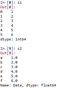
- Series的屬性:
- s2.axes。
- s2.dtype or s2.dtypes。
- s1.hasnans。
- s1.empty: 查看是否為空。
- s2.iloc[[0,1,2]], s2.iloc[np.arange(3)], s2.iloc[3:6] or s2.iloc[[True, False, True, True, False, True]]。
- 省略iloc依然可得到相同結果,e.g. s2[np.arange(3)], s2[list(range(0,6,2))]
- s2.loc['b'], s2.loc['b':]。
- iloc的index參數僅可用數字,所以s2.iloc['b']是錯的。loc的index參數僅可用index名稱,所以在此s2.loc[2:]是錯的。
- s1.iloc[:3]的意思是取前三個,而s1.loc[:3]的意思取到index為3止。
- s2.index: 等同s2.keys()。
- s2.is_monotonic, s2.is_monotonic_decreasing, s2.is_monotonic_increasing。
- s2.is_unique: 如果data內有重複資料則傳回false。
- s2.itemsize: s2.dtype/8。
- s2.nbytes: s2.itemsize*s2.size。
- s2.ndim。
- s2.shape。
- s2.size。
- s2.values: Return Series as ndarray or ndarray-like depending on the dtype。
- 上述屬性原則上多能用在DataFrame
Operations
- Series原則上與list, tuple, ndarray等類似,也能進行大部分運算。
import pandas as pd import numpy as np s1 = pd.Series([1,2,3,4,5,6]) s2 = pd.Series(np.arange(1,7), index = ['a','b','c','d','e','f'], dtype = float, name = "Data") dic = {'a':1, 'b':2, 'c':3, 'd':4, 'e':5} s3 = pd.Series(dic) items = ['a','b','c','d','e'] s4 = pd.Series(np.arange(1,6), index = items) s5 = pd.Series(np.random.randint(1, 100, 9))
- 改變其中的值: s1[0] = 100。
- 改變數值型態: s1.astype('float')。
- 基本運算(+,-,*,/,**,//,%): s1**2, s1/3。
- 若要進行s1+s2(s1.add(s2)),兩者的index相同者才會相加(e.g. s2+s3),index不同處則疊加。
- 若要疊加直接使用append >> s1.append(s2)。
- s2.combine(s3, lambda i, j: i if i==j else 0):combine兩個Series,函數須給兩參數,然後傳回一個傳回值。
- 數學函數: np.sin(s1),np.log(s1), np.sqrt(s1)。
- 使用agg(aggregate)將函數應用於Series上: s1.agg('min')或s1.agg(lambda x: x+2)或s1.agg(['min', 'max'])。
- 也可以使用apply: s1.apply(lambda x: x+2),s1.apply('sqrt'), s1.apply(['min','max'])。
- 也可以使用transform: s1.transform(lambda x:x+2)或s1.transform(lambda x:np.sqrt(x))。
- 或使用pipe: s1.pipe(np.min)或s1.pipe(min)或s1.pipe(np.sin)。
- s2.add(s3), s2.sub(s3),s2.mul(s3),s2.div(s3): s2+-*/s3(subtract, multiply, divide)。
- s1.mod(3): s1%3。
- s2.pow(s3): s2的s3次方。
- s2.prod()(或s2.product()): production of s2。
- s9 = pd.Series(np.random.rand(10)) >> s9.round(2): 取小數後2位四捨五入。
- 統計相關函數:
- s1.describe()。
- s1.count()。
- s1.max()。
- s1.min()。
- s1.mean()。
- s1.median()。
- corr(other, method='pearson', min_periods=None): correlation with `other` Series, excluding missing values。s1.corr(s5)或s1.corr(s5, 'pearson')或s1.corr(s5, 'kendall')。
- cov(other, min_periods=None):covariance with Series, excluding missing values。s1.cov(s5)
- diff(periods=1): discrete difference of object。
- s1.pct_change(): 前後元素的增減比例。
- mad(axis=None, skipna=None, level=None): mean absolute deviation。
- s5.std(): standard deviation。
- s2.ptp():最大跟最小值之差。
- s1.sample(3) or s1.sample(n=3): 隨機取三個元素。
- s5.sem(): unbiased standard error of the mean。
- s5.sum()。
- s5.var(): unbiased variance。
- 邏輯判斷: 判斷是否符合條件。
- s1>3: 傳回一個boolean陣列。若是s1[s1>3]則傳回符合條件(True)的Series。
- s1.clip(2,5),s1.clip_lower(2),s1.clip_upper(5): 將小於2的值變成2,大於5的值變成5。
- s1.isin(array): s1.isin([2,5]),傳回一個boolean陣列(值為2或5傳回True)。若是s1[s1.isin[2,5]]則傳回符合條件(True)的Series。
- s1.isnull(): 判斷是否為missing values(e.g. np.NaN)。
- s1.notnull(): 判斷是否不為missing values。
- all() & any(): Series.all(axis=0, bool_only=None, skipna=True, level=None, **kwargs)
ss = s1>3 ss.all() ss.any()
s6 = pd.Series(['a','b','a','c','b','d','a']) s6.duplicated() s6.duplicated(keep = 'first') s6.duplicated(keep = 'last') s6.duplicated(keep = False)
for i in s1.items(): print(i) for i,j in s1.items(): print(i,j)
- s1.get(2): 相當於s1[2] or s1.at[2]。
- s1.get_values(): 相當於s1.values。
- s1.get_dtype_counts(): 判斷各類型元素個數。
- s1.compress(s1>3): 等同s1[s1>3]。
- s1.between(2,5) & s1[s1.between(2,5)]: s1.between(2,5, inclusive=False)不包含判斷值。也可用於字串e.g. between('c','k')。
- s1.copy(): 建立物件的copy。
- s1.pop(0): 移除index為0之元素。
- s1.drop(3): 刪除index為3之元素。
- s1.drop_duplicates(): 刪除重複元件。
- s1.dropna(): 刪除missing values。
- groupby(by=None, axis=0, level=None, as_index=True, sort=True, group_keys=True, squeeze=False, **kwargs): s1.groupby(lambda x: x>3).mean()。
- s1.head(3): 選取前三元素。
- s1.tail(3): 選取後三元素。
- s2.map(s1): s1的值對應至s2或function應用到s2。
s = pd.Series([0, 1, np.NaN, 3, np.NaN]) ss = s.map("Amount: {}".format, na_action = None) # na_action = 'ignore' sss = s.map(lambda x: x**2)
- s1.add_prefix('item_')或s1.add_suffix('_item')。
- s1.reindex([1,3,5,2,'d','e'])。
- s1.rename(lambda x: x**2), s1.rename('demand'), s1.rename({0: 100, 1: 200})。
- s1.rename_axis('customers')or s1.rename_axis('customer', axis= 0): change axis in DataFrame。
- s1.set_axis(0, ['a', 'b', 'c','d','e','f']): 將s1的index改為第二個參數。
- unstack(level=-1, fill_value=None):用來將多重index轉換成DataFrame。
temp = pd.Series([1,2,3,4], index = pd.MultiIndex.from_product([['one','two'],['a','b']])) temp.unstack() temp.unstack(level=-1) temp.unstack(level=0)
s = pd.Series([0, 1, np.NaN, 3]) s.interpolate()
s7 = pd.Series(np.random.randint(1, 100, 9)) print(s5.argsort()) s8 = pd.Series(np.random.randint(1,30, 5), index = ['book','chair','key','printer','phone']) s8.sort_index() s8.sort_values()
- s7.argsort()傳回index的排序(非元素值的排序)。
- s8.sort_index()傳回一個Series,此Series根據index排序。
- 若使用s8.sort_index(ascending=False)>>降冪。
- 若使用s8.sort_index(inplace=True)>>直接排序s8(不需再指派給其他變數)。
- 若包含NaN且想將其排在上方,則使用s8.sort_index(na_position='first')。
- s8.sort_values()傳回一個Series,此Series根據value排序。
- 若使用s8.sort_values(ascending=False)>>降冪。
- 若使用s8.sort_values(inplace=True)>>直接排序s8(不需再指派給其他變數)。
- 若包含NaN且想將其排在上方,則使用s8.sort_values(na_position='first')。
- s5.to_clipboard(): 複製到system clipboard。
- s1.to_csv('temp.csv'): 寫到csv檔。
- s1.to_dict(): 轉為dict。
- s1.to_excel("data.xls",'Sheet1'): 寫到excel檔。
- s1.to_frame(): 轉換為dataframe。
- s5.to_json(): 轉換為JSON。
- s1.to_string()。
- s5.tolist(): 傳回values的list。
DataFrame
- DataFrame是多維陣列,原則上就是多個Series的組合,建立方式可為如下方式:
pandas2.py
datadic = {'cargo': ['computer','pen','keyboard','book','marker'], 'price': [35000,12,260,750,55], 'demand': [50,700,80,125,90]} df1 = pd.DataFrame(datadic) df2 = pd.DataFrame(datadic, columns=['cargo','price']) df2.index = ['class A', 'class B', 'class C', 'class D', 'class E']
- pandas.DataFrame(data=None, index=None, columns=None, dtype=None, copy=False)。
- 使用dict來建立,每一個column為一個Series。
- 使用index參數來改變index名稱(row),使用columns來改變column名稱。
- 原則上Series的參數屬性多可用在DataFrame,也有部分屬性僅適用於DataFrame。
- df1.columns, df1.index >> df1.axes >> df1.ndim。
- df1.shape >> df1.size。
- df1.info >> df1.values。
- df1.dtypes。
- df1.at[0,'demand'] <<>> df1['demand'][0] <<>> df1.iat[0,1]。
- df1.demand <<>> df1['demand']。
- df1[1:3], df1[lambda df: df.columns[0]]。
- iloc
- df1.iloc[[0,1,2]]
- df1.iloc[0]
- df1.iloc[0,1]
- df1.iloc[:,2]
- df1.iloc[[True, False, True, True, False]]
- df1.iloc[1:3,1:3]
- loc
- df1.loc[0]
- df1.loc[[0,1]]
- df1.loc[:,['cargo', 'price']]
- df1.loc[:, lambda df: ['cargo', 'price']]
- df1.demand.loc[[2,3,4]]
- df1.loc[[True, False, True, True, False]]
- df1.loc[df1['demand'] > 100]
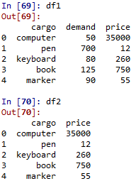
Operations
datadic = {'cargo': ['computer','pen','keyboard','book','marker'], 'price': [35000,12,260,750,55], 'demand': [50,700,80,125,90]} df1 = pd.DataFrame(datadic) df2 = pd.DataFrame(datadic, columns=['cargo','price']) df2.index = ['class A', 'class B', 'class C', 'class D', 'class E'] df3 = pd.DataFrame(np.random.randint(1,100, 16).reshape(4,4), index = ['a','b','c','d'], columns = ['one','two','three','four']) df4 = pd.DataFrame(np.random.randint(1,100, 16).reshape(4,4), index = ['a','b','c','d'], columns = ['one','two','three','four'])
- 適用於Series的方法大都可用於DataFrame,有的需要指派方向(軸),有些僅適用於DataFrame。
- df2.index.name = 'id',df2.columns.name = 'items': index與columns的名稱。
- 改變其中的值: df2['price'] = [36000, 15, 250, 800, 50], df2['price'][0] = 36500, df2.iloc[1,1] = 20, df3['one'] = 100。
- 新增一個column或row: df2['newColumn'] = 18或 df2['newColumn'] = [36000, 15, 250, 800, 50]; df2.loc['newRow'] = 36500 或 df2.loc['newRow']=[1,2,3,4,5]。
- 改變數值型態: df1['price'] = df1['price'].astype('float')。
- 基本運算
df1a = df1.reindex_like(df1) # 建立一個新的DataFrame df1b = df1.copy() # 也可建立一個新的DataFrame df1+df1a # 相加兩個DataFrame df1['price'] = df1['price'] + df1a['price'] # 相加兩個columns(or Series) df1['price'] = df1['price'] - df1a['price'] df1['price'] *3 df1['price'] /3 df1['price'] %3
- df5 = [df1, df4]: 疊加(與df1+df4不同)
- pd.concat([df3, df4]) or pd.concat([df3,df4], axis= 1, join_axes=[df3.index]): slightly different from [df3, df4]
- pd.merge(df3, df4, how='left', on=['one','two']):如果how='inner',需要row內容相同才會合併。如果how='outer'會疊加。
- join
df = pd.DataFrame(np.arange(12).reshape(4,3), index = ['a','b','e','f'], columns = ['five','six','seven']) df3.join(df) df3.join(df, how='inner') df3.join(df, how='outer') df3.join(df, how='left') df3.join(df, how='right')
- 使用agg(aggregate)將函數應用於Series上: df1['price'].agg('min')或df1['price'].agg(lambda x: x*2)或df1['price'].agg(['min','max'])。
- 也可以使用apply: df1['price'].apply(lambda x: x*2),df1['price'].apply('sqrt'), df1['price'].apply(['min','max'])。
- 也可以使用transform: df1['price'].transform('sqrt')或df1['price'].transform(lambda x: np.sqrt(x))。
- 或使用pipe: df1['price'].pipe(lambda x: np.sqrt(x))或df1['price'].pipe(np.min)或df1['price'].pipe(min)。
- df1['price'].add(df2['price']), df1['price'].sub(df2['price']),df1['price'].mul(df2['price']),df1['price'].div(df2['price']): df1['price']+-*/df2['price'](subtract, multiply, divide)。使用iloc[]來取得一個row的Series來進行row向的運算。
- 整個DataFrame的計算,與上述僅針對兩個Series不同:
s = pd.Series([1,2,3,4],index = df3.columns) df3-s
- 相當於每一個column都減去s內的對應值,其餘運算(+-*/)相同。
- 若是df3+df4,因為row跟col相同,所以對應元素會進行運算。
- df3.iloc[0]%13 vs. df3['one']%13。
- df3['one'].pow(df3['two']), or df7 = pd.DataFrame(np.arange(1,10).reshape(3,3))>>df7.iloc[1].pow(df7.iloc[0])。
- df3['one'].prod()(或df3['one'].product()): production of df3['one']。
- df2['rate']=[np.random.rand() for i in range(5)] >> df2['rate'].round(2): 取小數後2位四捨五入。
- df3.cummax(axis = 0) and df3.cummax(axis = 1):Return cumulative max。
- df3.cummin(axis = 0) and df3.cummin(axis = 1):Return cumulative min 。
- df3.cumprod(axis = 0 or 1): Return cumulative product。
- df3.cumsum(axis = 0 or 1): Return cumulative sum。
- df3.dot(df4.T) or df3.T.dot(df4): dot product。
- df3[df3 > 30].fillna(method = 'ffill') and df3[df3 > 30].fillna(method = 'bfill'): 往前與往後填滿NaN。See also >> df3[df3>30].fillna(0)。
- df1.T: 轉置矩陣,同df1.transpose()與np.transpose(df1)。
- df1.describe()。
- df1.count()。
- df1.max() & df1['price'].max()。
- df1.min() & df1['price'].min()。
- df1.mean() & df1['price'].mean()。
- df1.median() & df1['price'].median()。
- corr(other, method='pearson', min_periods=None): correlation with `other` Series, excluding missing values。df3['one'].corr(df3['two'])或df3['one'].corr(df3['two'], 'kendall')或df3['one'].corr(df4['two'])。
- df3.corrwith(df4): See also df3.corrwith(df4,axis=1)。
- cov(other, min_periods=None):covariance with Series, excluding missing values。df3['one'].cov(df3['two'])
- diff(periods=1): discrete difference of object。df3.diff()或df3['one'].diff()或df3.iloc[0].diff()或df3.T.diff()
- df3.pct_change()或df3['one'].pct_change(): 前後元素的增減比例。
- mad(axis=None, skipna=None, level=None): mean absolute deviation。df3.mad()或df3.mad(1)
- df3.std(): standard deviation。或df3['one'].std()或df3.iloc[0].std()
- df3['one'].ptp():最大跟最小值之差。
- df3.sample(3) or df3['one'].sample(3): 隨機取三個元素。
- df3.sem()或df3['one'].sem(): unbiased standard error of the mean。
- df3.sum()或df3['one'].sum()。
- df3.var()或df3['one'].var()或df3.T.var(): unbiased variance。
- df3 > 30: 傳回一個boolean陣列。若是df3[df3>30]則傳回符合條件(True)的DataFrame。
- df3.clip(10, 90),df3.clip(lower = 10),df3.clip(upper = 90): 將小於10的值變成10,大於90的值變成90。
- df3.isin([7, 81]), df3['one'].isin([7, 81]): 傳回一個boolean DataFrame or 陣列(值為7或81傳回True)。若是df3[df3.isin([7, 81])]則傳回符合條件(True)的DataFrame。。
- isnull(): 判斷是否為missing values(e.g. np.NaN),e.g. dfnan = df3[df3.isin([7, 81])] >> dfnan.isnull()。
- notnull(): 判斷是否不為missing values,dfnan.notnull()。
- all() & any(): Series.all(axis=0, bool_only=None, skipna=True, level=None, **kwargs),e.g.(df3<90).all()或(df3>90).any()
- duplicated(keep='first'): 判斷是否有重複。keep='first'表示判斷該元素之前是否有與其重複之元素,keep = 'last'表示判斷該元素之後是否有與其重複之元素,keep = False表示判斷該元素是否為重複元素。
df3['one'].duplicated() df3.loc['c'].duplicated() df3.loc['c'].duplicated('last') df3.loc['c'].duplicated(keep = False)
for i in df1.items(): print(i) for i in df1.columns: for j in df1.index: print(i,j,">>",df1[i][j])
- df1.get('cargo'): 相當於df1['cargo']。
- df1.at[0,'demand']: 相當於df1['demand'][0]或df1.loc[0].at['demand']或df1['demand'].at[0]或df1.get('demand').at[0]。
- df1.get_values(): see also df1.get('cargo').get_values()。
- df1.get_dtype_counts(): 判斷各類型元素個數。
- df1['price'].compress(df1['price']>100): 等同df1.get('price')[df1.get('price')>100]。
- df3.get('one').between(50,100) & df3['one'][df3.get('one').between(50,100)]: df1['cargo'].between('book','marker', inclusive=False)不包含判斷值。也可用於字串。
- df1_copy = df1.copy(): 建立物件的copy。
- df1_copy.pop('demand'): 移除column為demand之Series。Try del df1['price']。
- truncate(before=None, after=None, axis=None, copy=True): 移除前後,e.g.df1.truncate(before=1, after=3), df3.truncate(before='one', after='two', axis = 1)。
- df1_copy.drop(1): 刪除index為1之row。Try df1.drop('price', axis = 1)
- df5.drop_duplicates('B', 'first',inplace=False) or df5.drop_duplicates('B', 'last',inplace=False): 刪除column B中重複元素之row。
- (df3[df3<80]).dropna(): 刪除missing values所在之row。
- groupby(by=None, axis=0, level=None, as_index=True, sort=True, group_keys=True, squeeze=False, **kwargs):
df5 = pd.DataFrame({'One':['a','b','a','c','b','c'], 'Two':['i','i','j','j','k','k'], 'Three': np.arange(1,7), 'Four': np.random.randint(1,20,6)}) df5.groupby(['One']).first() df5.groupby(['One']).last() df5.groupby(['One']).sum() df5.groupby(['One','Two']).sum() df5.groupby(['One']).groups df5['Four'].groupby(df5['One']).sum() df5['Four'].groupby(df5['Three']>3).groups for name, group in df5.groupby('One'): print('Group name = ', name, '\n------------------') print(group)
- df1.head(3)): 選取前三元素,預設值為5。
- df1.tail(3): 選取後三元素。
- df3.applymap(fun): 將fun應用到df3的元素。也可以使用之前提及的agg, apply, transform, pipe等方式。
df3.applymap(lambda x: x**2) # same to df3**2 df3.applymap(lambda x: np.sin(x)) # same to np.sin(df3) or df3.applymap(np.sin)
- df1.filter(regex = 'e$') or df1.filter(regex = 'e+'): 使用regex選取column。
- df1.filter(like='3', axis = 0) or df1.filter(like='pri', axis = 1): 選擇包含3或pri之row或column。
- items, regex, 與like應分開使用。
- df1.columns.name = 'items'或df1.index.name = 'id':修改columns name。
- df1.add_prefix('item_')或s1.add_suffix('_item'):修改每一column的名稱。
- df1.reindex([1,3,2,0,4]):修改index的順序,若是給不同的index,內容會變成NaN。若是要重新命名index,使用df1.index = ['a','b','c','d','e']。
- df1.rename({'a':1,'b':2,'c':3,'d':4,'e':5}):可用來重新命名index。使用兩個mapper來改變row跟column的名稱,e.g. df1.rename({'a':'A'}, {'cargo':'ITEMS'})。
- df1.rename_axis({'a':1,'b':2}) or df1.rename_axis({'cargo':'items'}, axis=1): 可用來改變index或columns的名稱。
- df1.set_axis(0, [1,2,3,4,5]) and df1.set_axis(1, ['A','B','C']): 修改df1的index與column為第二個參數。
- df1.stack()與df1.unstack():將DataFrame轉換成多重index。
df6 = pd.DataFrame(np.random.randint(1,100, 16).reshape(4,4), index = [['A','A','B','B'],['boy','girl','boy','girl']], columns = [['Book','Book', 'Pen','Pen'],['red','blue','red','blue']]) df6_s = df6.stack() print(df6_s) print(df6_s.unstack()) df6_u = df6.unstack() print(df6_u) print(df6_u.stack()) df6.index.names = ['class', 'gender'] df6.columns.names = ['item','color'] df6.swaplevel('class','gender')
df1['demand'].argsort() df1.reindex([3,2,0,4,1]) df1.sort_index() df1.sort_values(by='demand')
- df1['demand'].argsort()傳回index的排序(非元素值的排序)。
- df1.sort_index()根據index排序,reindex用來重排index以方便排序。
- 若使用df1.sort_index(ascending=False)>>降冪。
- 若使用df1.sort_index(ascending=False, inplace=True)>>直接排序s8(不需再指派給其他變數)。
- df1.sort_values(by='demand')根據column demand的value排序。
- 若使用df1.sort_values(by='demand', ascending=False)>>降冪。
- 若使用df1.sort_values(by='demand', ascending=False, inplace=True)>>直接排序s8(不需再指派給其他變數)。
- df1.to_clipboard(): 複製到system clipboard。
- df1.to_csv('temp.csv') or df1.to_csv('temp.txt'): 寫到csv檔。pd.read_csv('temp.csv') or pd.read_csv('temp.csv', sep=',') or pd.read_csv('temp.csv', header = None) or pd.read_csv('temp.csv', names = ['id', 'info1', 'info2', 'info3'])
- df1.to_dict(): 轉為dict。
- to_html(): 。
htmlfile = open('ahtml.html','w') htmlfile.write(df1.to_html()) htmlfile.close() webdf = pd.read_html('ahtml.html') # give absolute dir(e.g. http://www.yahoo.com) to read other webpages
- df1.to_excel('data1.xls', 'sheet1'): 寫到excel檔。Read from excel: pd.read_excel('data1.xls'), pd.read_excel('data1.xls', 0), pd.read_excel('data1.xls', 'sheet1')
- df1.to_json(): 轉換為JSON。
- pickle(>>import pickle): df1.to_pickle('pkframe.pkl') >> pd.read_pickle('pkframe.pkl')。
- df1['price'].to_frame() or df1.loc[1].to_frame(): Series轉換為dataframe。
- df1.to_string()。
- df1['price'].tolist() or df1.loc[1].tolist(): 傳回column(row) values的list。
- to_sql。
from sqlalchemy import create_engine engine = create_engine('sqlite:///adb.db') df1.to_sql('dframe1', engine) df1_sql = pd.read_sql('dframe1', engine) print(df1_sql)
## use sqlite3 import sqlite3 query = """CREATE TABLE test(a VARCHAR(20), b VARCHAR(20), c REAL, d INTEGER);""" con = sqlite3.connect(':memory:') con.execute(query) con.commit() data = [('A','book',1,3), ('B','key',2,6), ('C','desk',8,9), ('D','pen',5,7)] stmt = "INSERT INTO test VALUES(?,?,?,?)" con.executemany(stmt, data) con.commit() cursor = con.execute('select * from test') rows = cursor.fetchall() print(rows) data1 = pd.DataFrame(rows) data2 = pd.DataFrame(rows, columns = ['class','item','value1','value2'])
results = np.random.randint(1,100, 100) bins = [0,20,40,60,80,100] cut1 = pd.cut(results, bins) cut2 = pd.cut(results, bins, labels = ['A','B','C','D','E']) cut3 = pd.cut(results, 5) print(pd.value_counts(cut1),"\n", pd.value_counts(cut2),'\n', pd.value_counts(cut3))
frame1 = pd.DataFrame(np.arange(1,17).reshape(4,4)) neworder = np.random.permutation(4) print(frame1.reindex(index = neworder)) # or use >> frame1.take(neworder)
idx = pd.date_range('1/1/2018', periods=12, freq='MS') df7 = pd.DataFrame(np.random.randint(1,100, 24).reshape(12,2), index = idx, columns = ['item1','item2'])
- 使用pd.date_range(start=None, end=None, periods=None, freq='D', tz=None, normalize=False, name=None, closed=None, **kwargs)方法。
- 也可以使用pd.date_range(start='1/1/2018',end='12/31/2018', freq='M')。
- 若使用pd.date_range(start='1/1/2018',end='12/31/2018'),沒有freq,內定為日,所以會有365個週期。freq有以下常用選擇:
- B: 上班日
- D: 日
- W: 周
- M: 月底
- SM: 月中
- BM: 上班月底
- MS: 月初
- SMS: 半月
- BMS: 上班月初
- Q: quarter end
- BQ: business quarter end
- QS: quarter start
- BQS: business quarter start
- A: 年底
- BA: 上班年底
- AS: 年初
- BAS: 上班年初
- BH: 上班小時
- H: 小時
- T, min: 分鐘
- S: 秒
- L, ms: 毫秒(milliseconds)
- U, us: microseconds
- N: nanoseconds
- 上述freq也可以加上數字,例如5D, 12H(每5日, 12小時)。
- normalize為True的話會先將start跟end轉化為當日0時。
- tz為時區。
- closed初始值為None,表示start跟end兩個時間點包含在區間,可改為left(左包含)或right(右包含)。
- 若是時間並非規則的
dates = [pd.Timestamp('2018-01-01'), pd.Timestamp('2018-01-13'), pd.Timestamp('2018-02-02')] df8 = pd.DataFrame([1,2,3], index = dates) # different from >> pd.DataFrame(dates, index=[1,2,3])
- 使用Timestamp()來建立時間。
- 原則上Timestamp()內的參數可以為以下形式:'1/1/2018','2018/01/01', '20180101', '2018.01.01', '01.01.2018', 'Jan 1, 2018'(通常為月日,若是不合理則自動改為日月。e.g. '12.13.2018' vs. '13.12.2018')。若是只有月分,可簡化為'2018-01','2018-02'等
- asfreq: 可用來改變freq,自動內插
df8.asfreq('D')
- 使用to_datetime建立DatetimeIndex
dt = pd.to_datetime(['2018/01/01 10:00', '2018/01/01 22:00']) s = pd.Series([1,2], dt) s.asfreq('H')
- 使用dt.year, dt.month, dt.day, dt.hour, dt.minute來取得個別參數。
- 使用dt[1]-dt[0]取得兩個時間之差。
- first & last (for TimeSeries): df7.first('3M'), df7.last('5M')。See also >> df7.head() & df7.tail(3)
- truncate: 去除前後。e.g. df7.truncate(before='2018-03-01', after='2018-10-01')。
Matplotlib
- Matplotlib可幫助我們繪製圖形,例如曲線圖長條圖等。使用時須先import matplotlib.pyplot這個模組。
pyplot1.py
import matplotlib.pyplot as plt
plt.plot([1,2,3,4])

- plot([x], y, [fmt], data=None, **kwargs)
- plot([x], y, [fmt], [x2], y2, [fmt2], ..., **kwargs)
import numpy as np
import pandas as pd
import matplotlib.pyplot as plt
x = np.arange(10,20)
y = pd.Series(np.random.randint(1,10,10))
plt.plot(x,y,'bo')
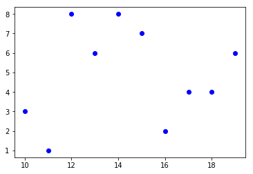
- 上例若是沒有給format('bo'),則會defaultly繪製折線圖。
- 顏色的format有許多選擇,e.g:
- b: blue
- g: green
- r: red
- c: cyan
- m: magenta
- y: yellow
- k: black
- w: white
- #rrggbb: 16進位法方式顯示,此時無法直接與形狀合用。須用關鍵字。
- 形狀的format亦有許多選擇,e.g.:
- '-' or 'solid
- '--' or 'dashed'
- '-.' or 'dashdot'
- ':' or dotted
- 'None' or '' or ' '
- '.'
- ','
- 'o'
- 'v'
- '^'
- '<'
- '>'
- '1'
- '2'
- '3'
- '4'
- '8'
- 's'
- 'p'
- '*'
- 'h'
- 'H'
- '+'
- 'x'
- 'X'
- 'D'
- 'd'
- '|'
- '_'
- r"$\alpha$"
- r"$\beta$"
- r"$\gamma$"
- r"$\sigma$"
- r"$\infty$"
- r"$\spadesuit$"
- r"$\heartsuit$"
- r"$\diamondsuit$"
- r"$\clubsuit$"
- r"$\bigodot$"
- r"$\bigotimes$"
- r"$\bigoplus$"
- r"$\imath$"
- r"$\bowtie$"
- r"$\bigtriangleup$"
- r"$\bigtriangledown$"
- r"$\oslash$"
- r"$\ast$"
- r"$\times$"
- r"$\circ$"
- r"$\bullet$"
- r"$\star$"
- r"$+$"
- r"$\Theta$"
- r"$\Xi$"
- r"$\Phi$"
- r"$\$$"
- r"$\#$"
- r"$\%$"
- r"$\S$"
- Plot的其他參數: 以下為部分參數
- color: color = "#ff00ff"。
- dash_capstyle: 'butt', 'round','projecting'。
- dash_joinstyle: 'miter', 'round','bevel'。
- dashes: dashes(on, off)。e.g. dashes(5,5)。
- drawstyle: 'default', 'steps', 'steps-pre', 'steps-mid', 'steps-post'。
- linestyle or ls: 'solid', 'dashed', 'dashdot', 'dotted', (offset, on-off-dash-seq) e.g. (10,(5,5,10,2)), '-', '--', '-.', ':', 'None','',' '。
- fillstyle: fill the marker。'full', 'left', 'right', 'bottom', 'top', 'none'。
- linewidth or lw: linewidth = 5。
- marker: marker = r"$\beta$"。
- alpha: alpha=0.5。
- markeredgecolor or mec: mec = 'blue'。
- markeredgewidth or mew: marker edge width,e.g. mew = 1.5。
- markerfacecoloralt or mfcalt: mfcalt='pink'。
- markerfacecolor or mfc: marker face color,e.g. mfc = "green"。
- markersize or ms: ms = 10。
- markevery: 每間隔幾個設置marker。'None', 'int', (a,b), slice, list/array, float。
- snap: 繪於格子點。snap=True(None)。
- solid_capstyle: 'butt', 'round','projecting'。
- solid_joinstyle: 'miter', 'round', 'bevel'。
關於線段(linestyle):
關於點(Marker):
其他特殊點(使用屬性marker, e.g. marker = r"$\alpha$"):
import numpy as np
import pandas as pd
import matplotlib.pyplot as plt
x = np.arange(10,20)
y = pd.Series(np.random.randint(1,10,10))
plt.plot(x,y,marker="o", color='blue', dash_capstyle="round",
drawstyle='steps', fillstyle='left', ls=(10,(5,3,5,5)),
mec = 'red', mew = 0.5, mfc = 'green', mfcalt = 'pink', ms = 20,
markevery = (1,2))
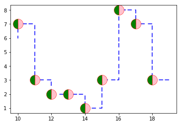
繪製多個圖型
- 只要將要繪製的圖型資料一一加入即可。
- plt.plot(x1,y1,'bo-',x2,y2,'r+--')會繪製兩條不同型式顏色的曲線。若是沒有加上'-'與'--',則只有點。
pyplot2.py
import numpy as np
import pandas as pd
import matplotlib.pyplot as plt
x1 = np.arange(10,20)
x2 = np.arange(1,11)
y1 = pd.Series(np.random.randint(1,10,10))
y2 = pd.Series(np.random.randint(10,20,10))
plt.plot(x1,y1,'bo-',x2,y2,'r+--')
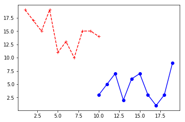
plt.plot(x1,y1,'bx-')
plt.plot(x2,y2,color='red', marker = 'o', mfc="b",mec='b', ls=':')
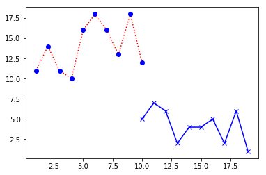
使用data繪製
- 若是有labeled的資料,例如dict,可以不抓取x,y,直接繪製。
- 使用plot([x], y, [fmt], data=None, **kwargs)其中的data。
import numpy as np
import pandas as pd
import matplotlib.pyplot as plt
x1 = np.arange(10,20)
x2 = np.arange(1,11)
y1 = pd.Series(np.random.randint(1,10,10))
y2 = pd.Series(np.random.randint(10,20,10))
dic1 = {'x1':x1, 'y1':y1}
plt.plot('x1','y1','bx-',data=dic1)
dic2 = {'x2':x2, 'y2':y2}
plt.plot('x2','y2',data=dic2, marker = 'o', mfc='b',mec='b',ls=':', color='r')
- plt.plot('x1','y1','bx-',data=dic1)中第一個參數'x1'為dict中的第一筆資料名稱,'y1'為第二筆資料名稱,這兩筆資料分別為x,y的值。
pyplot3.py
import numpy as np
import pandas as pd
import matplotlib.pyplot as plt
s = pd.Series(np.array([1,3,5,6,9]))
s.plot()
df = pd.DataFrame(np.random.randint(1,20,20).reshape(10,2))
df.plot() #也可以使用plt.plot(df.index, df)來繪製
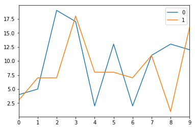
- plot()中一樣有許多參數可以使用來修飾圖型,在console輸入到左括號時會出現關鍵字提示,也可以使用help(s.plot)查詢,其中多個參數會在後面介紹。
- 若要使用df中第一個Series為x,第二個Series為y來繪圖,可以直接取出x與y然後使用plt.plot()來繪圖,其實若不嫌麻煩,都可以將資料取出,然後都使用plt.plot()來繪製即可。
dfx = df[0]
dfy = df[1]
plt.plot(dfx,dfy,'ro')
圖型的修飾
- 除了圖型顏色與線條,以下形式可以強化圖型的內容表示:
pyplot4.py
import numpy as np
import pandas as pd
import matplotlib.pyplot as plt
x = np.arange(5,25)
y = pd.Series(np.random.randint(5,45,20))
plt.figure(figsize=(8,6)) # set the size before other settings
plt.title("August", fontsize = 30, color='blue', fontname='castellar', pad = 10)
plt.xlabel('Day', color='g', fontsize = 15)
plt.ylabel('Temperature', color='c', fontsize = 15, fontname = 'Times New Roman')
plt.axis([0 ,30, 0, 50])
plt.grid(True)
plt.tick_params(axis='y', labelcolor='r')
for i in range(len(x)):
plt.text(x[i]+0.5, y[i]+0.5, y[i])
plt.minorticks_on()
plt.plot(x,y,'bo:', mfc = 'red', mec='red')
plt.legend(['oC'],loc=0)
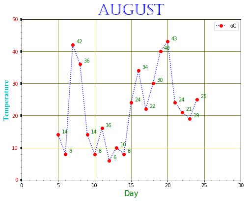
- plt.figure(figsize=(8,6))可設定圖型大小,但要放在其他設定之前。plt.figure()的部份其他屬性如下:
- figure(num=None, figsize=None, dpi=None, facecolor=None, edgecolor=None, frameon=True, FigureClass=
, clear=False, **kwargs) - 使用e.g. facecolor='#123456'與edgecolor='#abcdef'來改變背景顏色。
- dpi : integer, optional, default: None解析度,圖型大小跟著改變。
- plt.title()可建立圖型的title。
- fontdict: dictionary including fontsize, fontweight, verticalalignment(top, center, baseline), horizontalalignment(left, center, right)
- loc: title location, loc='left','center','right'。
- plt.xlabel()與plt.ylabel()可設定x,y軸的label。
- color: color='g'
- fontsize: fontsize = 15
- fontname: fontname = 'Times New Roman'
- plt.axis()用來設定axis的範圍。
- plt.grid(b=None, which='major', axis='both', **kwargs)。
- **kwargs可以使用line的參數,e.g. color="brown"。
- plt.tick_params(axis='both', **kwargs):改變tick的型態。
- plt.text(x, y, s, fontdict=None, withdash=False, **kwargs):可顯示文字於圖型。
- 在(x,y)位置顯示s文字。
- fontdict: 文字的性質,e.g. color='green'
- 若要顯示數學符號,可參考這個網頁
- plt.minorticks_on() vs plt.minorticks_off():開啟關閉minor ticks。
- plt.legend():顯示圖例。
- 定義在plot()之後。
- loc定義其位置,由0到10分別對應best, upper right, upper left, lower left, lower right, right,center left, center right, lower center, upper center, center。使用數字或文字皆可,亦即loc=1相等於loc='upper right'。可使用loc=0讓程式自己自動找最佳位置。
日期時間
- 如果某一軸是時間,因為時間需要較多文字顯示,顯示時可能會混雜在一起,例如:
pyplot5.py
import numpy as np
import pandas as pd
import matplotlib.pyplot as plt
dates = pd.date_range('01/01/2018', periods = 12, freq = 'D')
ydata = np.random.randint(1,30,12)
plt.plot(dates, ydata)

- 上圖可見x軸的日期互相交錯在一起,難以辨識。可以嘗試以下方式:
import numpy as np
import pandas as pd
import matplotlib.pyplot as plt
import matplotlib.dates as mdates
months = mdates.MonthLocator()
days = mdates.DayLocator()
timeFmt = mdates.DateFormatter('%m-%d')
dates = pd.date_range('01/01/2018', periods = 12, freq = '12D')
ydata = np.random.randint(1,30,12)
fig, ax = plt.subplots()
plt.plot(dates, ydata, 'rD', markersize='10')
ax.xaxis.set_major_locator(months)
ax.xaxis.set_major_formatter(timeFmt)
ax.xaxis.set_minor_locator(days)
繪製數學函數
- 數學函數繪製
pyplot6.py
import numpy as np
import matplotlib.pyplot as plt
import math
x = np.arange(-3*math.pi, 3*math.pi, 0.01)
y = np.sin(5*x)/x
plt.text(-7.5, 4, r'y=sin(5*x)/x', fontsize=12, color='b', bbox={'facecolor':'y','alpha':0.3})
plt.plot(x,y)
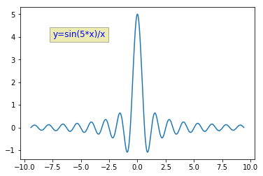
- 將x軸的tick顯示為pi,加上以下這一行。
plt.xticks([-3*math.pi, -2*math.pi, -math.pi, 0, math.pi, 2*math.pi, 3*math.pi],
[r'$-3\pi$', r'$-2\pi$', r'$-\pi$', r'$0$', r'$\pi$', r'$2\pi$', r'$3\pi$', ])
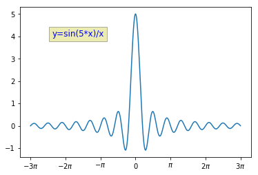
import numpy as np
import matplotlib.pyplot as plt
import math
x = np.arange(-3*math.pi, 3*math.pi, 0.01)
y5 = np.sin(5*x)/x
y3 = np.sin(3*x)/x
y1 = np.sin(x)/x
plt.text(-7.5, 4, r'y=sin(n*x)/x', fontsize=12, color='b', bbox={'facecolor':'y','alpha':0.3})
plt.plot(x,y1,'g-')
plt.plot(x,y3,'r:')
plt.plot(x,y5,'b--')
plt.xticks([-3*math.pi, -2*math.pi, -math.pi, 0, math.pi, 2*math.pi, 3*math.pi],
[r'$-3\pi$', r'$-2\pi$', r'$-\pi$', r'$0$', r'$\pi$', r'$2\pi$', r'$3\pi$', ])
plt.annotate(r'$\lim_{x\to 0}\frac{\sin(x)}{x}=1$',
xy = [0,1],
xycoords = 'data',
xytext = [30,30],
fontsize = 16,
textcoords = 'offset points',
arrowprops = dict(arrowstyle = "->", connectionstyle = "arc3, rad=.2"))
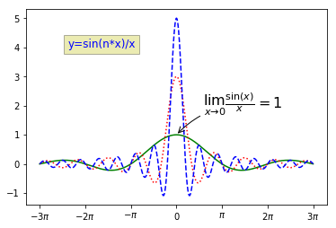
ax = plt.gca()
ax.spines['right'].set_visible(False)
ax.spines['top'].set_color('none')
ax.spines['bottom'].set_position(('data',0))
ax.spines['left'].set_position(('data',0))
ax.xaxis.set_ticks_position('bottom')
ax.yaxis.set_ticks_position('left')
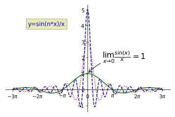
- 使用plt.gca()方法取得圖型脊柱(spines),共有四邊。
- 將上方(top)與右邊(right)脊柱設定為不可見或是無顏色,e.g.set_visible(False) or set_color('none')
- 移動左邊(left)與下方(bottom)的spines至預定位置,使用data關鍵字,位置為0,表示以資料為中心,若修改數字則會移動至其他位置。(將data改為outward將由原位置開始計算移動)
- 使用ax.xaxis.set_ticks_position('bottom')方式先取得xaxis,然後設定其ticks位置。
Multiple Figures & Axes
- 之前提過可以在一個圖表內繪製多個圖型,若是要繪製多個圖表並列做比較用途,可使用subplot。
import numpy as np
import matplotlib.pyplot as plt
x = np.arange(0,5,0.1)
y1 = np.sin(2*np.pi*x)
y2 = np.cos(2*np.pi*x)
plt.subplot(211)
plt.plot(x,y1,'b-.')
plt.subplot(212)
plt.plot(x,y2,'r--')
import numpy as np
import matplotlib.pyplot as plt
x = np.arange(0,5,0.1)
y1 = np.sin(2*np.pi*x)
y2 = np.cos(2*np.pi*x)
y3 = np.tan(2*np.pi*x)
plt.subplot(221, facecolor = 'lightgray')
plt.plot(x,y1,'b-.')
plt.subplot(2,2,2, polar = True)
plt.plot(x,y2,'r--')
plt.subplot(2,1,2)
plt.plot(x,y3,'g:')
- 嘗試改為(222)(224)(121)。
import numpy as np
import matplotlib.pyplot as plt
x = np.arange(0,5,0.1)
y1 = np.sin(2*np.pi*x)
y2 = np.cos(2*np.pi*x)
y3 = np.tan(2*np.pi*x)
y4 = np.log(x+1)
y5 = np.sin(np.pi*x)
grid = plt.GridSpec(3,3,wspace=0.5,hspace=0.5)
plt.subplot(grid[0,0:3])
plt.plot(x,y1,'b-.')
plt.subplot(grid[1,0:2])
plt.plot(x,y2,'r--')
plt.subplot(grid[2,0])
plt.plot(x,y3,'g:')
plt.subplot(grid[2,1])
plt.plot(x,y4,'b-')
plt.subplot(grid[1:3,2])
plt.plot(x,y5,'y-')
- 首先使用plt.GridSpec(3,3,wspace=0.5,hspace=0.5)取得格網物件,3,3分別代表row與column個數,wspace與hspace則代表寬高兩向的圖型空隙。
- 在subplot()方法中直接使用grid[]來表示該子圖所占的位置,e.g. 0, 0:3為第0row,0,1,2column。
顯示圖片
- 顯示圖片的方式:
import numpy as np
import matplotlib.pyplot as plt
from scipy.misc import imread
img1 = imread('./pic/flower1.jpg')
img2 = imread('./pic/flower2.jpg')
img2_tinted = img2*[1, 0.95, 0.9]
plt.subplot(1,2,1)
plt.imshow(img1)
plt.axis('off')
plt.subplot(122)
plt.imshow(np.uint8(img2_tinted))

Figures
- 除了可以使用前述的plot()方法來繪圖之外,Matplotlib尚提供其他方法來繪製其他形式的圖表。
- scatter(x, y, s=None, c=None, marker=None, cmap=None, norm=None, vmin=None, vmax=None, alpha=None, linewidths=None, verts=None, edgecolors=None, hold=None, data=None, **kwargs)[source]:scatter是散佈圖,當然也可以使用plot()來繪製散佈圖。
pyplot9.py
import numpy as np
import matplotlib.pyplot as plt
x = np.arange(10)
y = np.random.randint(1, 10, 10)
plt.figure(figsize=(8,6))
plt.scatter(x, y, color='red', marker=r'$\heartsuit$')
for i in range(len(x)):
t = "({},{})".format(str(x[i]),str(y[i]))
plt.text(x[i]+0.1, y[i]+0.2, t)
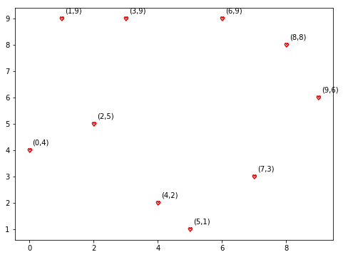
import numpy as np
import matplotlib.pyplot as plt
values = np.random.randn(1000)
n,bins,patches = plt.hist(values, bins=20, rwidth=0.8)
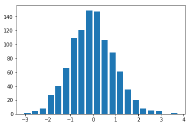
- bar(x, height, *, align='center', **kwargs)
- bar(x, height, width, *, align='center', **kwargs)
- bar(x, height, width, bottom, *, align='center', **kwargs)
import numpy as np
import matplotlib.pyplot as plt
x = [i for i in range(10)]#x = ['a','b','c','d','e','f','g','h','i','j']
y = np.random.randint(1,100,10)
plt.bar(x,y)
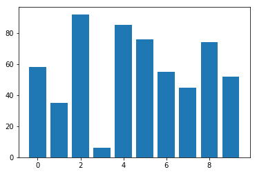
- barh(y, width, *, align='center', **kwargs)
- barh(y, width, height, *, align='center', **kwargs)
- barh(y, width, height, left, *, align='center', **kwargs)
import numpy as np
import matplotlib.pyplot as plt
x = [i for i in range(10)]#x = ['a','b','c','d','e','f','g','h','i','j']
y = np.random.randint(1,100,10)
plt.barh(x,y,height = 0.3,linewidth = 1,color='blue',edgecolor='red',log=True)
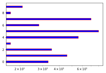
import numpy as np
import matplotlib.pyplot as plt
index = ['A','B','C','D','E','F','G','H','I','J']
values = np.random.randint(1,100,10)
err = [2 for i in range(10)]
plt.barh(index, values, xerr = err,
error_kw={'ecolor':'red', 'capsize':6},
alpha = 1, label = 'Some Data')
plt.legend(loc = 0)

import numpy as np
import matplotlib.pyplot as plt
index = np.arange(10)
value1 = np.random.randint(1,100,10)
value2 = np.random.randint(1,100,10)
value3 = np.random.randint(1,100,10)
err = [2 for i in range(10)]
plt.title('Multiseries Bar Chart', fontsize=20, color='b')
gap = 0.3
plt.bar(index, value1, gap, color='b', yerr=err, error_kw={'capsize':3}, label='Data 1')
plt.bar(index+gap, value2, gap, color='g', yerr=err, error_kw={'capsize':3}, label='Data 2')
plt.bar(index+2*gap, value3, gap, color='r', yerr=err, error_kw={'capsize':3}, label='Data 3')
plt.xticks(index+gap, index)
plt.legend(loc=0)
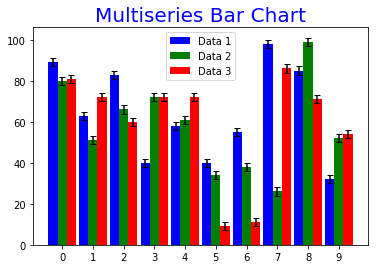
import numpy as np
import matplotlib.pyplot as plt
index = np.arange(5)
value1 = np.random.randint(1,20,5)
value2 = np.random.randint(1,20,5)
value3 = np.random.randint(1,20,5)
plt.title('Stacked Bar Chart', fontsize=20, color='b')
plt.bar(index, value1, color='b', label='Data 1')
plt.bar(index, value2, color='g', label='Data 2', bottom=value1)
plt.bar(index, value3, color='r', label='Data 3', bottom=value1+value2)
plt.legend(loc=0)
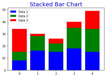
- 一樣使用plt.bar(plt.barh)來建立,只是要記得加上bottom=value1與bottom=value1+value2來表示資料的堆疊關係。餘皆相同。
- 若是要繪製橫向Stacked Bar Chart,要記得將bottom改為left。
- 上述的長條圖,都可以加上hatch來增加圖案,使得各筆資料間區隔更明顯。以下使用橫向Stack Bar Chart為例。
import numpy as np
import matplotlib.pyplot as plt
index = np.arange(5)
value1 = np.random.randint(1,20,5)
value2 = np.random.randint(1,20,5)
value3 = np.random.randint(1,20,5)
plt.title('Stacked Bar Chart with hatch', fontsize=20, color='b')
plt.barh(index, value1, color='b', edgecolor='r', label='Data 1', hatch="//")
plt.barh(index, value2, color='g', edgecolor='b', label='Data 2', left=value1, hatch="+++")
plt.barh(index, value3, color='r', edgecolor='g', label='Data 3', left=value1+value2, hatch="x")
plt.legend(loc=0)
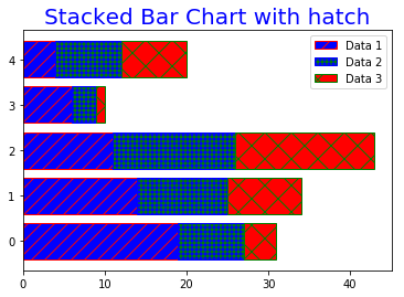
import numpy as np
import matplotlib.pyplot as plt
index = np.arange(1,9)
value1 = np.random.randint(1,10,8)
value2 = np.random.randint(1,10,8)
plt.ylim(-10,10)
plt.bar(index, value1, width=0.8, facecolor='r', edgecolor='g', linewidth=2, label='Data 1')
plt.bar(index, -value2, width=0.8, facecolor='b', edgecolor='k', linewidth=2, label='Data 2')
plt.grid(True)
for x,y in zip(index, value1):
plt.text(x, y+0.2, y, ha='center', va='bottom')
for x,y in zip(index, value2):
plt.text(x, -y-1.2, y, ha='center', va='bottom')
plt.legend(loc=0)
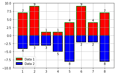
- 就是長條圖,把另一筆資料顯示在-y方向。
- 標示文字訊息時,使用zip()函數來取得座標,ha表示horizontalalignment,va表示verticalalignment。
import numpy as np
import matplotlib.pyplot as plt
label = ['Book', 'Pen', 'Key', 'Desk', 'Board']
amount = np.random.randint(1,100,5)
plt.title("Office Items", fontsize=20, color='b')
plt.pie(amount, labels=label, explode=[0.15,0,0,0,0], startangle=0, shadow=True, autopct='%.2f%%')
plt.axis('scaled') # scaled, tight, on, off, image, equal, auto, normal, square

- 跟之前類似需要x與y,在此使用label與amount表示。
- explode=[0.15,0,0,0,0]: 第一項資料(在此為Book)外突0.15。
- startangle=0: 從0度開始,逆時針方向。
- shadow=True: 加上陰影。
- autopct='%.2f%%': 自動計算比例,格式為小數後兩位。若要去除百分比號,可使用"%.2f"。
- plt.axis('scaled'): 改變圖型的軸,請自行嘗試其他選項。
import numpy as np
import matplotlib.pyplot as plt
x = np.arange(-3,3,0.01)
y = np.arange(-3,3,0.01)
m,n = np.meshgrid(x,y)
def f(p,q):
return (1-q**5+p**5)*np.exp(-p**2-q**2)
C = plt.contour(m, n, f(m,n), 8, colors='black')
plt.contourf(m, n, f(m,n), 16, alpha=0.8) # cmap=plt.cm.hot
plt.clabel(C, inline=1, fontsize=10)
plt.colorbar()
- 建立x,y兩筆資料,使用np.meshgrid(x,y)建立格子點座標。
- 建立一個函數,計算任一筆座標的對應高度。
- plt.contour(m, n, f(m,n), 8, colors='black'): 繪製等高線圖的輪廓,共8層。
- plt.contourf(m, n, f(m,n), 8, alpha=0.5): 使用顏色填滿等高線圖。
- plt.clabel(C, inline=1, fontsize=10): 標示等高線圖的數值,若inline=0表示連續線段,會與數值重疊。
- plt.colorbar(): 產生圖旁的顏色比例尺。
- 若是在plt.contourf()內加上參數cmap=plt.cm.hot,表示為溫度量圖,圖型會套用溫度量圖的設定。
- Check more information here。
- matplotlib.pyplot.polar(theta, r, **kwargs)
import numpy as np
import matplotlib.pyplot as plt
def genColor():
return '#'+''.join([np.random.choice(list('0123456789abcdef')) for i in range(6)])
N=8
theta = np.arange(0,2*np.pi,2*np.pi/N)
radii = np.random.randint(1,12,8)
plt.axes([0.05,0.05,0.95,0.95], polar=True)
plt.bar(theta, radii, width=(2*np.pi/N), bottom=0, color=[genColor() for i in range(N)])
- 為了使用顏色分辨各筆資料,建立genColor()函數來產生隨機顏色碼。
- plt.axes([0.05,0.05,0.95,0.95], polar=True): 繪製軸線,第一個參數為左上角及右下角座標,亦即可利用此來控制大小。polar須為True來形成圓形。
- plt.bar(theta, radii, width=(2*np.pi/N), bottom=0, color=[genColor() for i in range(N)]): 計算平均寬度讓每一項佔有一樣的弦寬,bottom=0表示連至圓心。
import numpy as np
import matplotlib.pyplot as plt
from mpl_toolkits.mplot3d import Axes3D
fig = plt.figure()
ax = Axes3D(fig)
theta = np.linspace(-4*np.pi, 4*np.pi, 100)
z = np.linspace(-2,2,100)
r = z**2+1
x = r*np.sin(theta)
y = r*np.cos(theta)
ax.plot(x, y, z, label='parametric curve', color='r')
ax.legend(loc=0, fontsize=12)
- 為了繪製3D圖型,需要from mpl_toolkits.mplot3d import Axes3D。
- ax = Axes3D(fig): 將figure cast成為3D物件。
- ax.plot(x, y, z, label='parametric curve', color='r'): 給x,y,z參數值即可繪製3D線形圖。
import numpy as np
import matplotlib.pyplot as plt
from mpl_toolkits.mplot3d import Axes3D
x1 = np.random.randint(10,20,100)
y1 = np.random.randint(10,20,100)
z1 = np.random.randint(10,30,100)
x2 = np.random.randint(10,20,100)
y2 = np.random.randint(30,40,100)
z2 = np.random.randint(30,50,100)
x3 = np.random.randint(70,80,100)
y3 = np.random.randint(10,20,100)
z3 = np.random.randint(30,50,100)
fig = plt.figure()
ax = Axes3D(fig)
ax.scatter(x1, y1, z1, color='g', marker='1')
ax.scatter(x2, y2, z2, color='r', marker='^')
ax.scatter(x3, y3, z3, color='b', marker='*')
ax.set_xlabel('X')
ax.set_ylabel('Y')
ax.set_zlabel('Z')
plt.title('3D Scatter', color='b', fontsize=20)
- 設計三組(x,y,z)座標,並分別使用ax.scatter()方法繪製散佈圖。
- 使用ax.set_xlabel('X')設定坐標軸的label。
import numpy as np
import matplotlib.pyplot as plt
from mpl_toolkits.mplot3d import Axes3D
x = np.arange(-5,5,0.25)
y = np.arange(-5,5,0.25)
x, y = np.meshgrid(x,y)
z = np.sin(np.sqrt(x**2+y**2))
fig = plt.figure()
ax = Axes3D(fig)
ax.plot_wireframe(x,y,z,rstride=1,cstride=1)
surf = ax.plot_surface(x,y,z,rstride=1, color='tomato', cmap=plt.cm.hot)#cmap=plt.cm.hot or cmap=plt.cm.coolwarm
fig.colorbar(surf, shrink=0.5, aspect = 15) # not needed if no cmap
ax.set_xlabel('X')
ax.set_ylabel('Y')
ax.set_zlabel('Z')
ax.view_init(elev=60, azim=125)
- ax.plot_wireframe(x,y,z,rstride=1,cstride=1): 繪製網格,若僅有此指令顯示圖型架構網格。
- ax.plot_surface(x,y,z,rstride=1, color='tomato'): 繪製表面。
- rstride=1表示row跨度,cstride=1表示column跨度,跨度越小表示線條越密。
- ax.view_init(elev=60, azim=125): 視角,elev上下旋轉,azim左右旋轉。
- cmap=plt.cm.hot: 將plt.com.hot之設定應用到圖型上。
- fig.colorbar(surf, shrink=0.5, aspect = 15): 若沒有cmap,則無作用。shrink=0.5控制長度,aspect = 15控制寬度。
import numpy as np
import matplotlib.pyplot as plt
from mpl_toolkits.mplot3d import Axes3D
fig = plt.figure()
ax = Axes3D(fig)
x = np.arange(4)
y = np.arange(5)
x, y = np.meshgrid(x,y)
x, y = x.ravel(), y.ravel()
'''
x = np.random.randint(1,20,20)
y = np.random.randint(1,20,20)
'''
z = x+y
bottom = np.zeros_like(z)
ax.bar3d(x,y,bottom, dx=0.5, dy=0.5,dz=z,color='g',shade = True)
ax.set_xlabel('X')
ax.set_ylabel('Y')
ax.set_zlabel('Z')
ax.view_init(elev=60, azim=125)
- 設計x,y,z的值,在此三者皆為1D-array(所以使用ravel(),可嘗試直接建立長度為20的array)。
- ax.bar3d(x,y,bottom, 0.5, 0.5,z,color='g',shade = True): dx與dy為x,y的寬度,z到dz為z的長度(柱子高度)。
import numpy as np
import matplotlib.pyplot as plt
from mpl_toolkits.mplot3d import Axes3D
x = np.arange(5)
y1 = np.random.randint(0,10,5)
y2 = np.random.randint(0,10,5)
y3 = np.random.randint(0,10,5)
z1 = np.random.randint(0,10,5)
z2 = np.random.randint(0,10,5)
z3 = np.random.randint(0,10,5)
fig = plt.figure()
ax = Axes3D(fig)
ax.bar(x,y1,z1,zdir='y',label='item 1')
ax.bar(x,y2,z2,zdir='y',label='item 2')
ax.bar(x,y3,z3,zdir='y',label='item 3')
ax.set_xlabel('X')
ax.set_ylabel('Y')
ax.set_zlabel('Z')
ax.legend(loc = 0)
- zdir='y': 表示以y的值當作z方向,若改為zdir='x'改用x的值。
with Pandas
- 之前提過Pandas中的Series與DataFrame皆可直接使用plot()方法來繪製圖型,但若是要繪製長條圖或其他圖型,則可使用參數關鍵字kind,e.g.
import numpy as np
import pandas as pd
df = pd.DataFrame(np.random.randint(1,20,12).reshape(6,2), index=['a','b','c','d','e','f'], columns=['Data 1','Data 2'])
df.plot(kind='bar', title='Data Frame', subplots=False, rot=0, yerr=[0.8 for i in range(6)], grid=True)
#df['Data 1'].plot(kind='pie', figsize=(6,6), explode=[0.15,0,0,0,0,0], autopct='%.2f%%') # equivalent to a Series
#df.loc['a'].plot(kind='pie')
- Series的kind可使用的選擇有: line, bar, barh, hist, box, kde, density, area, pie
- DataFrame的kind可使用的選擇有: line, bar, barh, hist, box, kde, density, area, pie, scatter, hexbin
- 這方式雖然便利,不過有些功能較少,例如無法改變title的格式,所以若是要較完整的功能,建議還是使用matplotlib。
Patches
- 若要繪製幾何圖型,例如矩形或是圓形等,可使用matplotlib.patches函式庫。其中包含了以下數種class(更多細節請參考官方網站):
- matplotlib.patches.Arc(xy, width, height, angle=0.0, theta1=0.0, theta2=360.0, **kwargs)
- matplotlib.patches.Arrow(x, y, dx, dy, width=1.0, **kwargs)
- matplotlib.patches.ArrowStyle[source]
- ArrowStyle.Fancy(head_length=.4, head_width=.4, tail_width=.4)
- ArrowStyle("Fancy", head_length=.4, head_width=.4, tail_width=.4)
- ArrowStyle("Fancy, head_length=.4, head_width=.4, tail_width=.4")
- matplotlib.patches.BoxStyle[source]
- BoxStyle.Round(pad=0.2)
- BoxStyle("Round", pad=0.2)
- BoxStyle("Round, pad=0.2")
- matplotlib.patches.Circle(xy, radius=5, **kwargs)
- matplotlib.patches.CirclePolygon(xy, radius=5, resolution=20, **kwargs)
- matplotlib.patches.ConnectionPatch(xyA, xyB, coordsA, coordsB=None, axesA=None, axesB=None, arrowstyle='-', arrow_transmuter=None, connectionstyle='arc3', connector=None, patchA=None, patchB=None, shrinkA=0.0, shrinkB=0.0, mutation_scale=10.0, mutation_aspect=None, clip_on=False, dpi_cor=1.0, **kwargs)
- matplotlib.patches.ConnectionStyle
- ConnectionStyle.Arc3(rad=0.2)
- ConnectionStyle("Arc3", rad=0.2)
- ConnectionStyle("Arc3, rad=0.2")
- matplotlib.patches.Ellipse(xy, width, height, angle=0.0, **kwargs)
- matplotlib.patches.FancyArrow(x, y, dx, dy, width=0.001, length_includes_head=False, head_width=None, head_length=None, shape='full', overhang=0, head_starts_at_zero=False, **kwargs)
- matplotlib.patches.FancyArrowPatch(posA=None, posB=None, path=None, arrowstyle='simple', arrow_transmuter=None, connectionstyle='arc3', connector=None, patchA=None, patchB=None, shrinkA=2, shrinkB=2, mutation_scale=1, mutation_aspect=None, dpi_cor=1, **kwargs)
- matplotlib.patches.FancyBboxPatch(xy, width, height, boxstyle='round', bbox_transmuter=None, mutation_scale=1.0, mutation_aspect=None, **kwargs)
- matplotlib.patches.Patch(edgecolor=None, facecolor=None, color=None, linewidth=None, linestyle=None, antialiased=None, hatch=None, fill=True, capstyle=None, joinstyle=None, **kwargs)
- matplotlib.patches.PathPatch(path, **kwargs)
- matplotlib.patches.Polygon(xy, closed=True, **kwargs)
- matplotlib.patches.Rectangle(xy, width, height, angle=0.0, **kwargs)
- matplotlib.patches.RegularPolygon(xy, numVertices, radius=5, orientation=0, **kwargs)
- matplotlib.patches.Shadow(patch, ox, oy, props=None, **kwargs)
- matplotlib.patches.Wedge(center, r, theta1, theta2, width=None, **kwargs)
- matplotlib.patches.YAArrow(figure, xytip, xybase, width=4, frac=0.1, headwidth=12, **kwargs)
Ellipse
- 以Ellipse為例。
- 橢圓的參數為xy(中心點)、width、height、angle(旋轉角度),請見下面的例子:
pyplot11.py
import numpy as np
import matplotlib.patches as pa
import matplotlib.pyplot as plt
num = 200 # the number of ellipse
def createEll():
ell = pa.Ellipse(xy=np.random.rand(2)*10,
width=np.random.rand(),
height=np.random.rand(),
angle=np.random.rand()*360)
return ell
ells = [createEll() for i in range(num)]
fig, ax = plt.subplots(subplot_kw={'aspect':'equal'})
fig.set_size_inches(6,6)
for i in ells:
ax.add_artist(i)
i.set_alpha(np.random.rand())
i.set_facecolor(np.random.rand(3))
ax.set_xlim(0,10)
ax.set_ylim(0,10)
plt.title("Ellipses", fontsize=20, color='b')
- createEll(): 用來建立一個ellipse的物件。
- fig, ax = plt.subplots(subplot_kw={'aspect':'equal'}): 將圖型分為圖案(fig)與軸(ax>兩個物件。
- ax.add_artist(i): 將ellipse(i)加入圖型中。
- i.set_alpha(np.random.rand()): 設定transparency。
- i.set_facecolor(np.random.rand(3)): 設定顏色。
- ax.set_xlim(0,10): 設定x軸的範圍。
Web Scraping
requests
import requests r = requests.get("http://www2.nkust.edu.tw/~shanhuen") print(r.text) print(r.status_code) print(r.reason) print(r.request) print(r.request.url) print(r.request.headers)------ url with query string ------
import requests url = 'http://www.webscrapingfordatascience.com/paramhttp/' parameters = { 'query': 'a query with /, spaces and?&' } r = requests.get(url, params=parameters) print(r.url) print(r.text)
BeautifulSoup
import first(from bs4 import BeautifulSoup)BeautifulSoup(html_contents, "html.parser")
- html.parser: a decent built-in Python parser
- lxml: very fast, requires extra installation
- html5lib: parse web page in exactly the same way as a web browser does, but is a bit slower
find & find_all(findAll)
find(name, attrs, recursive, string, **keywords) find_all(name, attrs, recursive, string, limit, **keywords)
-
attr: print(soup.find('', {'id': 'p-logo'}))
-
recursive: True: look into through the deepest leaves
False: only look at direct child elements -
limit: 搜尋個數,僅用於find_all(),在find()中為1。若找不到符合元素,傳回空list。 -
**kewwords: find(id='myid')
等同於 find(attrs={'id': 'myid'})”find(class_='myclass')
記得要使用class_,不能使用class。
import requests from bs4 import BeautifulSoup import re soup = BeautifulSoup(requests.get('http://www2.nkust.edu.tw/~shanhuen/css/css_7.html').text, 'html.parser') firsth1 = soup.find("h1") print(firsth1.name, " ", firsth1.contents, " ", str(firsth1), " ", firsth1.text, " ", firsth1.getText(), " ", firsth1.attrs) links = soup.find_all("a", href=True) images = soup.find_all("img", src=True) ps = soup.find_all('p') images2 = soup.find_all('img', src=re.compile('\.png$')) for pp in soup.findAll('p', class_="css7_8"): print(pp) print(soup.find_all(True)) #check all tags
More on BeautifulSoup
html_soup.find('h1') html_soup.find(['h1', 'h2'])
html_soup.find(re.compile('^h'))兩者效果相同。
- find_parent & find_parents
- find_next_sibling & find_next_siblings
- find_previous_sibling & find_previous_siblings
- find_next & find_all_next use the next_elements
- find_previous & find_all_previous
print(soup.select('a')) print(soup.select('.css7_8')) print(soup.select("div.gallery.des")) # 同時是class gallery與class des的div print(soup.select('div.gallery, div.des')) # class gallery or class des print(soup.select('a[href^="http://www.nkust.edu.tw"]')) print(soup.select('a[href!="http://www.nkust.edu.tw"]')) print(soup.select("div.gallery>a")) for d in soup.select('div.gallery, div.des'): print(d.text)
get vs. post
Press F12 to check if the form method is get or post first.- get: Same with metioned above
r = requests.get(url) print(r.text)
- post: use the following method like
formdata = { 'name': 'Tom', 'gender': 'Male', 'occupation': 'Student', 'comments': 'None' } r = requests.post(url, data=formdata) print(r.text)
r = requests.post(url, params={'type': 'student'}, data=formdata)或是說
paramdata = {'name': 'Totally Not Tom'} formdata = {'name': 'Tom'} r = requests.post(url, params=paramdata, data=formdata)
cookies & session
欲查form中有類似login資料,使用如下語法:session = requests.Session() r = session.post(url) r = session.post(url, params={'p':'login'}, data={'username':'name','password':'abc'}) r = session.get(url, params={'p':'protected'}) print(r.text) # use session.cookies.clear() to clean a session if you need it
Binary Data
例如取得圖片,可以使用如下程式碼:url = "http://www2.nkust.edu.tw/~shanhuen/css/images/img1.jpg" r = requests.get(url, stream=True) with open("image.jpg", 'wb') as f: for chunk in r.iter_content(chunk_size=4096): f.write(chunk)現在可以在資料夾內看到圖片image.jpg。
JSON
欲取得json資料,至https://www.591.com.tw/點擊租屋>F12>XHR,觀察response應有json資料。在Name選擇一個鏈結,在Headers中copy Request URL內容,即為url變數內容。url = "https://rent.591.com.tw/home/data/listExposure?type=1&post_id=7286438" r = requests.get(url) print(r.json()) print(r.json().get('msg'))
JavaScript
使用Selenium:- 首先安裝Selenium,使用指令
pip install selenium - 下載WebDriver,for Chrome:到以下網站https://sites.google.com/a/chromium.org/chromedriver/downloads,下載適合你的電腦版本的WebDriver(在Chrome選項選擇說明>關於Google Chrome可看到你的版本,亦可更新版本)。
- 選好版本點入,選擇OS類型然後下載。檔案放置在與你程式碼相同的資料夾,解壓縮後出現chromedriver.ext檔案。
from selenium import webdriver url = 'http://www2.nkust.edu.tw/~shanhuen/css/css_7.html' driver = webdriver.Chrome() driver.get(url) input('按ENTER關閉視窗') driver.quit()現在可以根據以下方法來取得元件:
- find_element_by_id
- find_element_by_name
- find_element_by_xpath
- find_element_by_link_text
- find_element_by_partial_link_text
- find_element_by_tag_name
- find_element_by_class_name
- find_element_by_css_selector
- nodename selects all nodes with the name “nodename”;
- / selects from the root node;
- // can be used to skip multiple levels of nodes and search through alldescendants to perform a selection;
- . selects the current node;
- .. selects the parent of the current node;
- @ selects attributes.
from selenium import webdriver url = 'http://www2.nkust.edu.tw/~shanhuen/css/css_7.html' driver = webdriver.Chrome() driver.get(url) for c in driver.find_elements_by_class_name('htmlcode'): print(c.text) input('按ENTER關閉視窗') driver.quit()若是需要給一點時間讓JavaScript執行完畢,可以增加等待時間,例如加上:
driver.implicitly_wait(10)
Geo Pandas
GeoPandas Installation
-
使用conda安裝:
conda install --channel conda-forge geopandas -
接下來測試一下,打開jupyter,輸入以下指令:
import geopandas as gpd world = gpd.read_file(gpd.datasets.get_path('naturalearth_lowres')) ax = world.plot(figsize=(20,20))
顯然使用前須import geopandas,若安裝成功應會顯示一個世界地圖。輸入print(world.head())
查看資料內容。
Basic Instructions
首先練習繪製世界地圖:import geopandas as gpd world = gpd.read_file(gpd.datasets.get_path('naturalearth_lowres')) ax = world.plot(figsize=(20,20))因為資料是pandas,所以可以使用例如loc或是iloc來取得資料,而GeoPandas還提供另一個方式(cx)來取得切片資料,標準型態為
southWorld = world.cx[:, :0] southWorld.plot(figsize=(10, 5))東半球資料:
eastWorld = world.cx[0:, :] eastWorld.plot(figsize=(10, 5))繪製包含重要城市之世界地圖:
world = gpd.read_file(gpd.datasets.get_path('naturalearth_lowres')) cities = gpd.read_file(gpd.datasets.get_path('naturalearth_cities')) ax = world.plot(figsize=(20,20)) cities.plot(ax=ax, color='y', markersize=20)根據某欄位來調配地圖顏色:
print(world.columns) world.plot(column='pop_est')加上Legend:
import geopandas as gpd import matplotlib.pyplot as plt from mpl_toolkits.axes_grid1 import make_axes_locatable world = gpd.read_file(gpd.datasets.get_path('naturalearth_lowres')) cities = gpd.read_file(gpd.datasets.get_path('naturalearth_cities')) fig, ax = plt.subplots(1,1,figsize=(20,20)) divider = make_axes_locatable(ax) cax = divider.append_axes("right", size="5%", pad=0.1) world.plot(ax=ax, column='pop_est', legend=True, cax=cax) cities.plot(ax=ax, color='r', markersize=5) plt.show()加上legend=True就會出現legend,不過大小跟圖並不匹配,所以額外導入
divider = make_axes_locatable(ax) cax = divider.append_axes("right", size="5%", pad=0.1)並在plot()內加上cax=cax參數,可以得到對應大小的legend。
另一個調色的方式是使用cmap:
world.plot(ax=ax, column='pop_est', cmap='plasma', legend=True, cax=cax) cities.plot(ax=ax, markersize=5, cmap='hot')crs:指的是座標對應系統(projection),可以使用例如world.crs來查詢(常見的代碼為epsg=4326),若是有多個圖層的圖須讓crs一致,可以使用例如如下的方式修改它。
world = gpd.GeoDataFrame(world,crs={'init','epsg:3395'})Geometry:可在地圖上額外繪製點線或多邊形。記得需先導入
gdf1 = gpd.GeoDataFrame({'geometry':[Point(0, 0), Point(100, 50)], 'attributes':[1,2]}) gdf1.plot(ax=ax, markersize=50, color='r')再來設計幾個多邊形:
p1 = Polygon([(0,0),(1,0),(1,1)]) p2 = Polygon([(0,0),(1,0),(1,1),(0,1)]) p3 = Polygon([(2,0),(3,0),(3,1),(2,1)]) g = gpd.GeoSeries([p1,p2,p3]) print(g)計算多邊形面積:
print(g.area) print(p1.area)使用g.buffer(distance=0.5)來傳回一個GeoSeries物件,表示原來每個物件在固定距離內的所有點。使用g.plot()繪圖。
g = g.buffer(distance=0.5) print(g) g.plot(color='b')
Set Operations
當地圖中元件重疊時,我們可以利用集合的概念來取得其交集、聯集、差集等。舉例說明如下,首先先設計幾個簡單的多邊形然後繪圖:import geopandas as gpd from shapely.geometry import Polygon p1 = gpd.GeoSeries([Polygon([(0,0),(2,0),(2,2),(0,2)]),Polygon([(2,2),(4,2),(4,4),(2,4)])]) p2 = gpd.GeoSeries([Polygon([(1,1),(3,1),(3,3),(1,3)]),Polygon([(3,3),(5,3),(5,5),(3,5)])]) df1 = gpd.GeoDataFrame({'geometry':p1, 'id':[1,2]}) df2 = gpd.GeoDataFrame({'geometry':p2, 'id':[1,2]}) ax = df1.plot(color='b') df2.plot(ax=ax, color='green', alpha=0.6)接下來繪製聯集的圖(
union = gpd.overlay(df1, df2, how='union') print(union) ax=union.plot(alpha=0.8, cmap='gist_rainbow') df1.plot(ax=ax, facecolor='none', edgecolor='k') df2.plot(ax=ax, facecolor='none', edgecolor='k')
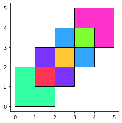 再來試交集(
intersection = gpd.overlay(df1, df2, how='intersection') print(intersection) ax=intersection.plot(alpha=0.8, cmap='gist_rainbow') df1.plot(ax=ax, facecolor='none', edgecolor='k') df2.plot(ax=ax, facecolor='none', edgecolor='k')
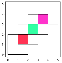 差集(
差集(symDiff = gpd.overlay(df1, df2, how='symmetric_difference') print(symDiff) ax=symDiff.plot(alpha=0.8, cmap='gist_rainbow') df1.plot(ax=ax, facecolor='none', edgecolor='k') df2.plot(ax=ax, facecolor='none', edgecolor='k')
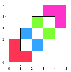 再試聯集減df2(
difference = gpd.overlay(df1, df2, how='difference') print(difference ) ax=difference.plot(alpha=0.8, cmap='gist_rainbow') df1.plot(ax=ax, facecolor='none', edgecolor='k') df2.plot(ax=ax, facecolor='none', edgecolor='k')
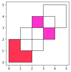 僅顯示聯集之後的df1(
identity = gpd.overlay(df1, df2, how='identity') print(identity ) ax=identity.plot(alpha=0.8, cmap='gist_rainbow') df1.plot(ax=ax, facecolor='none', edgecolor='k') df2.plot(ax=ax, facecolor='none', edgecolor='k')
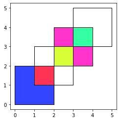 使用世界地圖練習:
world = gpd.read_file(gpd.datasets.get_path('naturalearth_lowres')) cities = gpd.read_file(gpd.datasets.get_path('naturalearth_cities')) countries = world[['geometry', 'name']] # 僅取兩欄 cities['geometry']= cities.buffer(2) # 城市的buffer=2,由點變成polygon intersection = gpd.overlay(countries, cities, how='intersection') #print(intersection) ax=intersection.plot(figsize=(20,20), alpha=0.8, cmap='gist_rainbow') countries.plot(ax=ax, facecolor='none', edgecolor='k') cities.plot(ax=ax, facecolor='none', edgecolor='k')

dissolve
使用dissolve()來群組資料,例如:import geopandas as gpd world = gpd.read_file(gpd.datasets.get_path('naturalearth_lowres')) world = world[['continent','geometry','pop_est']] #選取其中三欄 continents = world.dissolve(by='continent',aggfunc='min') # first(default),last,min,max,sum,mean,median ax=continents.plot(figsize=(15,15),column='pop_est', cmap='rainbow_r') continents.head()

merging data
合併資料(使用merge & sjoin):world = gpd.read_file(gpd.datasets.get_path('naturalearth_lowres')) cities = gpd.read_file(gpd.datasets.get_path('naturalearth_cities')) country_shapes = world[['geometry','iso_a3']] country_names = world[['name','iso_a3']] country_shapes = country_shapes.merge(country_names, on='iso_a3') #print(country_shapes.head()) countries = world[['geometry','name']] countries = countries.rename(columns={'name':'country'}) cities_with_country = gpd.sjoin(cities, countries, how='inner', op='intersects') print(cities_with_country.head())
使用外部資料
取得shape file資料(e.g. 台鐵資料)import geopandas as gpd rail = gpd.read_file('E:\\NKFUST\\www\\PythonTutorialHtml\\GeoPandas\\codes\\Rail.shp',encoding='utf-8') print(rail)rail原則上就是個dataframe,做為GeoDataFrame最主要的就是多了個geometry欄位,看一下內容,分別使用以下指令:
rail.head()
type(rail)
ax = rail.plot(figsize=(10,10), edgecolor='k')有多個shape file,e.g. 鄉鎮市區界線+村里界圖,使用如下語法畫在一個圖上:
df1 = gpd.read_file('E:\\NKFUST\www\PythonTutorialHtml\GeoPandas\codes\map2\\TOWN_MOI_1070330.shp',encoding='utf-8') df2 = gpd.read_file('E:\\NKFUST\www\PythonTutorialHtml\GeoPandas\codes\map2\\VILLAGE_MOI_1070330.shp',encoding='utf-8') ax = df2.plot(figsize=(30,30), edgecolor='w') df1.plot(ax=ax, edgecolor='r', alpha=0.35)
 Set operation:
import geopandas as gpd from shapely.geometry import Point, Polygon, LineString df1 = gpd.read_file('E:\\NKFUST\www\PythonTutorialHtml\GeoPandas\codes\map2\\TOWN_MOI_1070330.shp',encoding='utf-8') df2 = gpd.read_file('E:\\NKFUST\www\PythonTutorialHtml\GeoPandas\codes\map2\\VILLAGE_MOI_1070330.shp',encoding='utf-8') points = gpd.GeoDataFrame({'geometry':[Point(120, 23),Point(121, 24),Point(122, 25)]}) points = points.buffer(0.5) points = gpd.GeoDataFrame({'geometry':points}) points.crs = df1.crs difference = gpd.overlay(df1, points, how='difference') #print(intersection) ax=difference.plot(figsize=(20,20), cmap='flag') df1.plot(ax=ax, facecolor='none', edgecolor='r', alpha=0.3) df2.plot(ax=ax, facecolor='none', edgecolor='b', alpha=0.3)

BaseMap
BaseMap Installation
此列指令會建立設計的特定環境,名為eq_env,並確認此project的環境不會與其他project相互影響。此外如果package之前已經安裝過,可確認他們在此環境可以使用。接下來使用以下指令來啟動環境:
若要結束此環境,輸入以下指令:
接下來設計一個最簡單的例子來測試看是否環境設定成功:
from mpl_toolkits.basemap import Basemap import matplotlib.pyplot as plt import numpy as np worldmap = Basemap() worldmap.drawcoastlines() plt.show()現在在conda(需開啟環境,在指令前會看到eq_env)內輸入執行指令:
Attributions
在之前例子中,因為要繪製basemap,所以顯然需要導入(import)相關的package。接著呼叫Basemap()方法來建立地圖物件,然後呼叫內定的drawcoastlines()方法來繪製海岸線。最後使用plt.show()方法顯示。而其中方法可以加上其他屬性來改變圖形外觀,如下:worldmap = Basemap(projection='ortho', lat_0=23, lon_0=122, resolution='l', area_thresh=1000.0) worldmap.drawmapboundary(fill_color="aqua") worldmap.fillcontinents(color='#9af0e3', lake_color='blue') worldmap.drawcoastlines() plt.show()參數應該很容易理解,其中resolution內建有兩個選擇,crude(c)與low(l),若是想要有其他選擇(intermediate, high, full)則需使用
至於projection參數的值則有許多,e.q. cyl(default, Cylindrical Equidistant projection)、ortho、robin、aeqd、nsper 等。有些則需要搭配其他參數方能顯示(ortho需搭配lat_0與lon_0參數),或例如gnom需搭配寬(width)高(height):
worldmap = Basemap(projection='gnom', lat_0=23, lon_0=122, resolution='l', area_thresh=1000.0, width=15.e6, height=15.e6)另一個僅顯示部分區域的繪圖方式為tmerc,須提供lower-left跟upper-right corners的座標。:
worldmap = Basemap(projection='tmerc', lat_0=23, lon_0=122, resolution='l', area_thresh=1000.0, llcrnrlon=119.5, llcrnrlat=21.5, urcrnrlon=122.5, urcrnrlat=25.5)再另一個方式是使用nsper,此方法須以lat_0與lon_0為中心,給定左下與右上距離來繪製,如下:
worldmap = Basemap(projection='nsper', lat_0=23, lon_0=122, resolution='l', satellite_height=3000000.0, llcrnrx = -500000, llcrnry=-500000, urcrnrx=3000000, urcrnry=3000000)
Basic Functions
- 畫點:
x,y=worldmap(122,22) worldmap.plot(x,y,marker='D', color='m')
點的形狀見matplotlib或參考此網頁,而顏色則可參考此網頁。 若是要繪製的點超過一個,可以將座標存於list,然後使用scatter()方法。xs = [102, 112, 122, 132, 142] ys = [2, 12, 22, 32, 42] x, y = worldmap(xs, ys) worldmap.scatter(x, y, marker='D', color='b')
也可以使用plot()方式,但是會出現相連的線(與matplotlib相同,因為其實就是matplotlib)。
- 計算地圖上的點位置:inverse為False表示輸入為經緯度。
print(worldmap(10, 50)) print(worldmap(2573995.595313374, 11462906.414487308, inverse=True))
Basemap methods
使用方法前當然需要先有Basemap物件:mpl_toolkits.basemap.Basemap(llcrnrlon=None, llcrnrlat=None, urcrnrlon=None, urcrnrlat=None, llcrnrx=None, llcrnry=None, urcrnrx=None, urcrnry=None, width=None, height=None, projection='cyl', resolution='c', area_thresh=None, rsphere=6370997.0, ellps=None, lat_ts=None, lat_1=None, lat_2=None, lat_0=None, lon_0=None, lon_1=None, lon_2=None, o_lon_p=None, o_lat_p=None, k_0=None, no_rot=False, suppress_ticks=True, satellite_height=35786000, boundinglat=None, fix_aspect=True, anchor='C', celestial=False, round=False, epsg=None, ax=None)
接著使用matplotlib繪製annotation,例如:
from mpl_toolkits.basemap import Basemap import matplotlib.pyplot as plt worldmap = Basemap(projection='ortho', lat_0=22.6, lon_0=120.3) worldmap.drawmapboundary(fill_color="aqua") worldmap.fillcontinents(color='#9af0e3', lake_color='blue') worldmap.drawcoastlines() x, y = worldmap(120.3, 22.6) x2, y2 = (50, 20) plt.annotate('KaoHsiung', xy = (x, y), xycoords='data', xytext=(x2, y2), textcoords='offset points', color='r', arrowprops=dict(arrowstyle="fancy", color='g')) x2, y2 = worldmap(100, 10) plt.annotate('KaoHsiung', xy=(x,y), xycoords='data', xytext=(x2, y2), textcoords='data', arrowprops=dict(arrowstyle="->")) plt.show()
See more examples on Basemap2.py
PyQt
Qt是跨平台的視窗程式庫(GUI Library),PyQt就是Python+Qt,也就是使用Python來設計Qt視窗程式。要使用之前首先當然是安裝,請參考官網內容。幸運的是我們使用anaconda,PyQt5是預設安裝好的,因此可以直接盡情地使用。- 先看個例子:
from PyQt5.QtWidgets import QApplication , QLabel app = QApplication([]) label = QLabel('Hello, World') label.show() app.exec_()- 首先我們需要import PyQt5.QtWidgets,這個模組包含各種widget,而因為我們此處僅需要使用到QApplication與QLabel這兩個,所以僅導入此兩種。
- QApplication繼承自QGuiApplication,主要用來控制視窗的形成與關閉以及視窗事件等,且提供必要的函數來建立QWidget物件。每一個GUI需要一個且僅一個QGuiApplication物件。在建構時,其輸入引數為指令列參數,因為目前沒有指令列參數,所以給一個空白的list。也可以導入sys,然後給sys.argv作為輸入引數,因為它也是一個空白的list。
- QLabel()可以產生一個label物件,此處使用它的建構子之一如下:
QLabel(str, parent: QWidget = None, flags: Union[Qt.WindowFlags, Qt.WindowType] = Qt.WindowFlags())給一個str做為顯示文字。另一個建構子則是沒有str。接著使用label.show()來讓其顯示在視窗內。 - 最後的app.exec_()表示要求Qt接手並讓app持續工作直到使用者關閉為止。
- 接著嘗試稍作修改,建立一個完全陽春的空白視窗。
import sys import PyQt5.QtWidgets as wg def myWin(): app = wg.QApplication(sys.argv) # sys.argv >> [''] w = wg.QWidget() # 沒有指定parent的QWidget物件 >> 作為視窗使用 w.show() sys.exit(app.exec_()) ## same to app.exec_() if __name__ == '__main__': myWin()- 原則上幾乎與前一個程式碼相同,只是使用空白QWidget物件代替QLabel。基本三步驟:QApplication(sys.argv)、QWidget()建立與顯示、exec_()。接著我們使用各式函數來控制視窗外觀。
import sys import PyQt5.QtWidgets as wg from PyQt5.QtGui import QIcon, QPalette, QColor def myWin(): app = wg.QApplication(sys.argv) # sys.argv >> [''] w = wg.QWidget() # 沒有指定parent的QWidget物件 >> 作為視窗使用 w.setWindowTitle("PyQt5") # 設定視窗的title w.setGeometry(100,100,200,200) # 左上角座標, 右下角座標 w.move(200, 200) # 新的左上角座標 w.resize(300, 300) # 設定視窗寬高 # 設定icon需先import QIcon >> QIcon(路徑) w.setWindowIcon(QIcon('../RandomTalk/pics/icon.png')) # 設定背景顏色,需先import QPalette, QColor pa = app.palette() # 建立palette物件 pa.setColor(QPalette.Window, QColor("blue")) # or QPalette.Background >> 指定顏色位置 app.setPalette(pa) # 設定pa為app的palette w.show() sys.exit(app.exec_()) ## same to app.exec_() if __name__ == '__main__': myWin() - 接著加入label來顯示文字。
import sys import PyQt5.QtWidgets as wg from PyQt5.QtGui import QIcon, QFont class myWin(wg.QMainWindow): def __init__(self): super().__init__() self.app = wg.QApplication(sys.argv) # sys.argv >> [''] w = wg.QWidget() # 沒有指定parent的QWidget物件 >> 作為視窗使用 w.setWindowTitle("PyQt5") # 設定視窗的title w.setGeometry(100,100,300,300) # 左上角座標, 右下角座標 w.move(200, 200) # 新的左上角座標 w.resize(500, 500) # 設定視窗寬高 w.setStyleSheet("background-color: pink") # 設定icon需先import QIcon >> QIcon(路徑) w.setWindowIcon(QIcon('../RandomTalk/pics/icon.png')) ############ b = wg.QLabel(w) b.setText("Hello World!") # b.setAutoFillBackground(True) # 需設計背景充滿來設計背景顏色 b.setFont(QFont("Roman times",20,QFont.Bold)) b.setFixedWidth(200) b.setFixedHeight(100) b.move(100, 100) b.setStyleSheet("background-color: lightgreen; color: red") ############ w.show() sys.exit(self.app.exec_()) ## same to app.exec_() if __name__ == '__main__': win = myWin() - PyQt5有多個modules,包括QtCore、QtGui、QtWidgets、QtMultimedia、QtBluetooth、QtNetwork、QtPositioning、Enginio、QtWebSockets、QtWebEngine、QtWebEngineCore、QtWebEngineWidgets、QtXml、QtSvg、QtSql、QtTest等。
- 原則上幾乎與前一個程式碼相同,只是使用空白QWidget物件代替QLabel。基本三步驟:QApplication(sys.argv)、QWidget()建立與顯示、exec_()。接著我們使用各式函數來控制視窗外觀。
- 加入Button。
import sys import PyQt5.QtWidgets as wg from PyQt5.QtGui import QIcon, QFont class myWin(wg.QMainWindow): def __init__(self): super().__init__() self.app = wg.QApplication(sys.argv) # sys.argv >> [''] w = wg.QWidget() # 沒有指定parent的QWidget物件 >> 作為視窗使用 btn = wg.QPushButton("click", w) # QPushButton(str, parent: QWidget = None) btn.move(50, 50) btn.clicked.connect(self.fun1) # 連結button與對應函數 wg.QToolTip.setFont(QFont('SansSerif', 20, QFont.Bold)) aBtn = wg.QPushButton("Square", w) aBtn.move(50, 100) aBtn.setToolTip('button tool tip') aBtn.clicked.connect(lambda : print(self.area(5, 7))) ############ w.show() sys.exit(self.app.exec_()) ## same to app.exec_() def fun1(self): print("fun1 is executed.") def area(self, width, height): return width*height if __name__ == '__main__': win = myWin() - QBoxLayout:Layout Management可以如前所述的使用move()來安排widget的位置。此外可以使用其他方式,如QBoxLayout、QGridLayout或QFormLayout。
import sys import PyQt5.QtWidgets as wg class myWin(wg.QMainWindow): def __init__(self): super().__init__() self.app = wg.QApplication(sys.argv) # sys.argv >> [''] w = wg.QWidget() # 沒有指定parent的QWidget物件 >> 作為視窗使用 w.setGeometry(100, 100, 300, 300) # w.resize(500, 500) btn = wg.QPushButton("click", w) # QPushButton(str, parent: QWidget = None) btn.clicked.connect(self.fun1) # 連結button與對應函數 aBtn = wg.QPushButton("Square", w) aBtn.clicked.connect(lambda : print(self.area(5, 7))) vbox = wg.QVBoxLayout() # 使用Box Layout vbox.addWidget(btn) # addWidget: 加入widget vbox.addWidget(aBtn) vbox.addStretch() # stretchable:stretch之前加入的widget w.setLayout(vbox) # 設定layout為vbox ############ w.show() sys.exit(self.app.exec_()) ## same to app.exec_() def fun1(self): print("fun1 is executed.") def area(self, width, height): return width*height if __name__ == '__main__': win = myWin() - 如果要水平配置,使用QHBoxLayout()。
hbox = wg.QHBoxLayout() # 使用Box Layout hbox.addWidget(btn) # addWidget: 加入widget hbox.addWidget(aBtn) hbox.addStretch() # stretchable:stretch之前加入的widget w.setLayout(hbox) # 設定layout為vbox - nested。
import sys import PyQt5.QtWidgets as wg class myWin(wg.QMainWindow): def __init__(self): super().__init__() self.app = wg.QApplication(sys.argv) # sys.argv >> [''] w = wg.QWidget() # 沒有指定parent的QWidget物件 >> 作為視窗使用 # w.setGeometry(100, 100, 300, 300) w.resize(500, 500) btn1 = wg.QPushButton("click") # QPushButton(str, parent: QWidget = None) btn1.clicked.connect(self.fun1) # 連結button與對應函數 btn2 = wg.QPushButton("Square") btn2.clicked.connect(lambda : print(self.area(5, 7))) btn3 = wg.QPushButton("btn3") btn4 = wg.QPushButton("btn4") vbox = wg.QVBoxLayout() # 使用verticle Box Layout vbox.addWidget(btn3) # addWidget: 加入widget vbox.addStretch() # stretchable:stretch之前加入的widget vbox.addWidget(btn4) hbox = wg.QHBoxLayout() # 使用horizon Box Layout hbox.addWidget(btn1) # addWidget: 加入widget hbox.addStretch() # stretchable:stretch之前加入的widget hbox.addWidget(btn2) # vbox.addStretch() vbox.addLayout(hbox) # 將vhox加入到vbox w.setLayout(vbox) # 設定window layout為vbox ############ w.show() sys.exit(self.app.exec_()) ## same to app.exec_() def fun1(self): print("fun1 is executed.") def area(self, width, height): return width*height if __name__ == '__main__': win = myWin() - QGridLayout。
import sys import PyQt5.QtWidgets as wg class myWin(wg.QMainWindow): def __init__(self): super().__init__() self.app = wg.QApplication(sys.argv) # sys.argv >> [''] win = wg.QWidget() # 沒有指定parent的QWidget物件 >> 作為視窗使用 grid = wg.QGridLayout() # b1 = wg.QPushButton("b1") # b2 = wg.QPushButton("b2") # grid.addWidget(b1) # grid.addWidget(b2) for i in range(5): for j in range(5): grid.addWidget(wg.QPushButton(f"b{i}{j}"), i, j) # addWidget(widget, row, col) win.setLayout(grid) ############ win.show() sys.exit(self.app.exec_()) ## same to app.exec_() def fun1(self): print("fun1 is executed.") def area(self, width, height): return width*height if __name__ == '__main__': win = myWin()- 與box layout合併。
import sys import PyQt5.QtWidgets as wg from PyQt5.QtCore import * class myWin(wg.QMainWindow): def __init__(self): super().__init__() self.app = wg.QApplication(sys.argv) # sys.argv >> [''] win = wg.QWidget() # 沒有指定parent的QWidget物件 >> 作為視窗使用 top = wg.QLabel("Top") top.setStyleSheet("background-color: blue; color: white") top.setAlignment(Qt.AlignCenter) # or AlignRight from QtCore buttom = wg.QLabel("Buttom") buttom.setStyleSheet("background-color: blue; color: white") buttom.setAlignment(Qt.AlignCenter) # or AlignRight from QtCore grid = wg.QGridLayout() for i in range(5): for j in range(5): grid.addWidget(wg.QPushButton(f"b{i}{j}"), i, j) # addWidget(widget, row, col) vbox = wg.QVBoxLayout() vbox.addWidget(top) vbox.addLayout(grid) vbox.addStretch() vbox.addWidget(buttom) win.setLayout(vbox) ############ win.show() sys.exit(self.app.exec_()) ## same to app.exec_() def fun1(self): print("fun1 is executed.") def area(self, width, height): return width*height if __name__ == '__main__': win = myWin()
- 與box layout合併。
- QFormLayout使用addRow()方法來加入widget、str或layout,方法有以下幾種:
- addRow(self, QWidget, QWidget)
- addRow(self, QWidget, QLayout)
- addRow(self, str, QWidget)
- addRow(self, str, QLayout)
- addRow(self, QWidget)
- addRow(self, QLayout)
import sys import PyQt5.QtWidgets as wg from PyQt5.QtCore import * class myWin(wg.QMainWindow): def __init__(self): super().__init__() self.app = wg.QApplication(sys.argv) # sys.argv >> [''] win = wg.QWidget() # 沒有指定parent的QWidget物件 >> 作為視窗使用 top = wg.QLabel("Top") top.setStyleSheet("background-color: blue; color: white") top.setAlignment(Qt.AlignCenter) # or AlignRight from QtCore buttom = wg.QLabel("Buttom") buttom.setStyleSheet("background-color: blue; color: white") buttom.setAlignment(Qt.AlignCenter) # or AlignRight from QtCore lab_a = wg.QLabel("a") lab_a.setFixedWidth(100) lab_a.setStyleSheet("border: 1px solid black") lab_b = wg.QLabel("b") lab_b.setFixedWidth(100) lab_b.setStyleSheet("border: 1px solid blue") lab_c = wg.QLabel("c") lab_c.setFixedWidth(100) lab_c.setStyleSheet("border: 1px solid green") box = wg.QHBoxLayout() box.addWidget(lab_a) box.addWidget(lab_b) box.addWidget(lab_c) box.addStretch() fLay = wg.QFormLayout() fLay.addRow(top, wg.QPushButton("btn1")) # add a row fLay.addRow(wg.QPushButton("btn2"), buttom) # add a row fLay.addRow("Str: ", wg.QPushButton("btn3")) fLay.addRow(box) win.setLayout(fLay) ############ win.show() sys.exit(self.app.exec_()) ## same to app.exec_() def fun1(self): print("fun1 is executed.") def area(self, width, height): return width*height if __name__ == '__main__': win = myWin() - Pyqt包含多個widgets,例如:QLabel、QLineEdit、QPushButton、QRadioButton、QCheckBox、QComboBox、QSpinBox、QSlider、QMenuBar、QToolBar、QInputDialog、QFontDialog、QFileDialog、QTab、、QStacked、QSplitter、QDock、QStatusBar、QList、QScrollBar、QCalendar。
import sys import PyQt5.QtWidgets as wg from PyQt5.QtCore import * from PyQt5.QtGui import * class myWin(wg.QMainWindow): def __init__(self): super().__init__() self.app = wg.QApplication(sys.argv) # sys.argv >> [''] win = wg.QWidget() # 沒有指定parent的QWidget物件 >> 作為視窗使用 self.label = wg.QLabel("QLabel") ## lineEdit self.lineEdit = wg.QLineEdit ("Default text") self.lineEdit.returnPressed.connect(lambda: self.returnPressed(self.lineEdit.text())) ## Radio buttons inside a QVBoxLayout hboxRadio = wg.QHBoxLayout() rBtn1 = wg.QRadioButton("One") rBtn2 = wg.QRadioButton("Two") hboxRadio.addWidget(rBtn1) hboxRadio.addWidget(rBtn2) rBtn1.toggled.connect(lambda:self.rBtnState(rBtn1)) rBtn2.toggled.connect(lambda:self.rBtnState(rBtn2)) ## Check box hboxCheck = wg.QHBoxLayout() box1 = wg.QCheckBox("Maserati") box1.setChecked(True) box1.stateChanged.connect(lambda:self.boxState(box1)) box2 = wg.QCheckBox("Benz") box2.toggled.connect(lambda:self.boxState(box2)) box3 = wg.QCheckBox("Porsche") box3.toggled.connect(lambda:self.boxState(box3)) hboxCheck.addWidget(box1) hboxCheck.addWidget(box2) hboxCheck.addWidget(box3) ## QComboBox() self.combo = wg.QComboBox() self.combo.addItem("Python") self.combo.addItem("PyQt") self.combo.addItems(["C", "C++", "C#"]) self.combo.currentIndexChanged.connect(self.comboselection) ## QSpinBox() vboxSpin = wg.QVBoxLayout() self.showSpin = wg.QLabel("Year:") self.showSpin.setAlignment(Qt.AlignCenter) self.showSpin.setStyleSheet("border: 1px solid blue") self.spin = wg.QSpinBox() self.spin.setRange(1990, 2050) self.spin.valueChanged.connect(self.spinValue) vboxSpin.addWidget(self.showSpin) vboxSpin.addWidget(self.spin) ## QMenuBar menuBox = wg.QHBoxLayout() bar = self.menuBar() file = bar.addMenu("File") ## add one menu file.addAction("New") save = wg.QAction("save", self) file.addAction(save) edit = file.addMenu("Edit") ## add one menu edit.addAction("copy") edit.addAction("paste") toQuit = wg.QAction("Quit", self) bar.addAction(toQuit) ## add one action as menu menuBox.addWidget(bar) ## toolbar toolbar = self.addToolBar("File") # set a tool bar self.addToolBar("File") ## add the tool bar to win # add a new Action into toolbar ## QAction is inside PyQt5.QtGui newfile = wg.QAction(QIcon("new.png"),"new",self) toolbar.addAction(newfile) # add a open Action into toolbar openfile = wg.QAction(QIcon("open.jpg"),"open",self) toolbar.addAction(openfile) # add a save Action into toolbar savefile = wg.QAction(QIcon("save.jpg"),"save",self) toolbar.addAction(savefile) toolbar.actionTriggered[wg.QAction].connect(self.toolbarpressed) toolBox = wg.QVBoxLayout() toolBox.addWidget(toolbar) ## win layout fLay = wg.QFormLayout() fLay.addRow("Menu", menuBox) # add a row fLay.addRow("QLabel", self.label) # add a row fLay.addRow("QLineEdit ", self.lineEdit) # add a row fLay.addRow("QRadioButton ", hboxRadio) # add a row fLay.addRow("QCheckBox", hboxCheck) # add a row fLay.addRow("QComboBox", self.combo) # add a row fLay.addRow("QSpinBox", vboxSpin) # add a row fLay.addRow("QToolBar", toolBox) # add a row win.setLayout(fLay) ############ win.show() sys.exit(self.app.exec_()) ## same to app.exec_() def returnPressed(self, text): self.label.setText(f"{text}") def rBtnState(self, b): if b.text() == "One": if b.isChecked() == True: self.label.setText(f"{b.text()}") if b.text() == "Two": if b.isChecked() == True: self.label.setText(f"{b.text()}") def boxState(self, b): if b.text() == "Maserati": if b.isChecked() == True: print("Maserati is chosen.") else: print("Maserati is not chose.") if b.text() == "Benz": if b.isChecked() == True: print("Benz is chosen.") else: print("Benz is not chose.") if b.text() == "Porsche": if b.isChecked() == True: self.label.setText("Porsche is chosen.") else: self.label.setText("Porsche is not chose.") def comboselection(self, i): for c in range(self.combo.count()): # count() > Retrieves number of items in the collection print(self.combo.itemText(c)) # print(f"currently selected: {i} > {self.combo.currentText()}") # same to the following line print(f"currently selected: {self.combo.currentIndex()} > {self.combo.currentText()}") def spinValue(self): self.showSpin.setText(f"Year:{self.spin.value()}") def toolbarpressed(self, btn): print(f"You pressed: {btn.text()}") if __name__ == '__main__': win = myWin()- 更多網路上的介紹。
- QDialog。
import sys import PyQt5.QtWidgets as wg from PyQt5.QtCore import * from PyQt5.QtGui import * class myWin(wg.QMainWindow): def __init__(self): super().__init__() self.app = wg.QApplication(sys.argv) # sys.argv >> [''] win = wg.QWidget() # 沒有指定parent的QWidget物件 >> 作為視窗使用 btn = wg.QPushButton("click", win) btn.move(100, 100) btn.clicked.connect(self.showDialog) ############ win.show() sys.exit(self.app.exec_()) ## same to app.exec_() def showDialog(self): dialog = wg.QDialog() ## define a dialog def closeDialog(): ## function for close dialog dialog.close() b1 = wg.QPushButton("ok",dialog) b1.move(50,50) b1.clicked.connect(closeDialog) # close dialog by click ok dialog.setWindowTitle("Dialog") #dialog.setWindowModality(Qt.ApplicationModal) # 關閉dialog後才能與父視窗互動(關閉),不過這行指令似乎可有可無 dialog.exec_() if __name__ == '__main__': win = myWin() - QMessageBox。
import sys import PyQt5.QtWidgets as wg class myWin(wg.QMainWindow): def __init__(self): super().__init__() self.app = wg.QApplication(sys.argv) # sys.argv >> [''] win = wg.QWidget() # 沒有指定parent的QWidget物件 >> 作為視窗使用 btn = wg.QPushButton("message", win) btn.move(100, 100) btn.clicked.connect(self.showMessageDialog) ############ win.show() sys.exit(self.app.exec_()) ## same to app.exec_() def showMessageDialog(self): mbox = wg.QMessageBox() btnMessage = lambda i: print(f"You pressed: {i.text()}") mbox.setIcon(wg.QMessageBox.Information) ## Question, Information, Warning, Critical mbox.setText("Main message") mbox.setInformativeText("Additional information") mbox.setWindowTitle("Message Box") mbox.setDetailedText("The details are as follows: more details") mbox.setStandardButtons(wg.QMessageBox.Ok | wg.QMessageBox.Cancel) mbox.buttonClicked.connect(btnMessage) mbox.exec_() if __name__ == '__main__': win = myWin() - MDI (Multiple Document Interface)使用較少記憶體控制多個視窗,使用QMdiArea wwidget。Child window是QMdiSubWindow物件。
import sys import PyQt5.QtWidgets as wg class myWin(wg.QMainWindow): def __init__(self): super().__init__() self.app = wg.QApplication(sys.argv) # sys.argv >> [''] self.subCount = 0 self.mdi = wg.QMdiArea() # 建立多視窗顯示區域 self.setCentralWidget(self.mdi) # 設mdi為主視窗 bar = self.menuBar() file = bar.addMenu("File") file.addAction("New") file.triggered[wg.QAction].connect(self.windowaction) winArrange = bar.addMenu("Window") winArrange.addAction("cascade") winArrange.addAction("Tiled") winArrange.triggered[wg.QAction].connect(self.windowaction) ############ self.setWindowTitle("MDI demo") self.show() sys.exit(self.app.exec_()) ## same to app.exec_() def windowaction(self, q): if q.text() == "New": self.subCount = self.subCount+1 sub = wg.QMdiSubWindow() # 產生sub window sub.setWidget(wg.QTextEdit()) # 設定QTextEdit widget sub.setWindowTitle(f"sub window {self.subCount}") self.mdi.addSubWindow(sub) # add sub window to mdi(QMdiArea) sub.show() # 顯示sub window if q.text() == "cascade": self.mdi.cascadeSubWindows() if q.text() == "Tiled": self.mdi.tileSubWindows() if __name__ == '__main__': win = myWin() - Drawing API
import sys import PyQt5.QtWidgets as wg from PyQt5.QtGui import * ## QPainter from PyQt5.QtCore import * ## Qt class myWin(wg.QMainWindow): def __init__(self): super().__init__() self.app = wg.QApplication(sys.argv) # sys.argv >> [''] win = wg.QWidget() self.setGeometry(100, 100, 800, 600) self.paintEvent(win) ############ self.setWindowTitle("Drawing API") self.show() sys.exit(self.app.exec_()) ## same to app.exec_() def paintEvent(self, win): qp = QPainter() qp.begin(self) qp.setPen(QColor("red")) # 設定畫筆顏色 qp.setFont(QFont('Arial', 20)) # 設定字型 qp.drawText(50,50, "hello Python") # draw text > (x,y,text) qp.drawArc(100, 300, 200, 500, 100, 500) qp.setPen(QColor('blue')) qp.drawLine(10,100,100,100) # line (x1, y1, x2, y2) qp.drawRect(10,150,150,100) # rect (x1, y1, x2, y2) qp.setPen(QColor('red')) qp.drawEllipse(300,300,100,50) # ellipse > (x1, y1, xx, yy) qp.drawPixmap(220,10,QPixmap("save.jpg")) qp.fillRect(20,175,130,70,QBrush(Qt.SolidPattern)) qp.end() if __name__ == '__main__': win = myWin()- Methods: begin()、drawArc()、drawEllipse()、drawLine()、drawPixmap()、drwaPolygon()、drawRect()、drawText()、fillRect()、setBrush()、setPen()。
- 關於QPixmap用法:
import sys from PyQt5.QtWidgets import * from PyQt5.QtGui import * ## QPainter from PyQt5.QtCore import * ## Qt class myWin(QWidget): def __init__(self): super().__init__() label = QLabel(self) label.setStyleSheet("border: 2px solid red;") pic = QPixmap("save.jpg") label.setPixmap(pic) label.resize(pic.width(),pic.height()) pic.save("abc.png") # 將QPixmap儲存為圖檔 ############ self.setWindowTitle("Pixmap") self.show() if __name__ == '__main__': app = QApplication(sys.argv) # sys.argv >> [''] win = myWin() app.exec_()
- Database
import sys from PyQt5.QtSql import * from PyQt5.QtWidgets import * from PyQt5.QtGui import * from PyQt5.QtCore import * class myWin(QWidget): def __init__(self): super().__init__() # 增加一個database db = QSqlDatabase.addDatabase('QSQLITE') db.setDatabaseName('sportsdatabase.db') ## table model self.model = QSqlTableModel() self.delrow = -1 self.initializeModel() ## 建立一個table view view1 = self.createView("Table Model (View 1)") view1.clicked.connect(self.findrow) # 將view加入layout layout = QVBoxLayout() layout.addWidget(view1) ## 加入add與del之button button = QPushButton("Add a row") button.clicked.connect(self.addrow) layout.addWidget(button) btn1 = QPushButton("del a row") btn1.clicked.connect(lambda: self.model.removeRow(view1.currentIndex().row())) layout.addWidget(btn1) self.setLayout(layout) ############ self.setWindowTitle("Database") self.show() def initializeModel(self): """ * 設定QSqlTableModel Returns ------- None. """ self.model.setTable('sportsmen') self.model.setEditStrategy(QSqlTableModel.OnFieldChange) self.model.select() self.model.setHeaderData(0, Qt.Horizontal, "ID") self.model.setHeaderData(1, Qt.Horizontal, "First name") self.model.setHeaderData(2, Qt.Horizontal, "Last name") def createView(self, title): """ * 建立一個Table view並設定其model為QSqlTableModel """ view = QTableView() view.setModel(self.model) view.setWindowTitle(title) return view def addrow(self): print (self.model.rowCount()) ret = self.model.insertRows(self.model.rowCount(), 1) print (ret) def findrow(self, i): self.delrow = i.row() if __name__ == '__main__': app = QApplication(sys.argv) # sys.argv >> [''] win = myWin() app.exec_()- PyQt5包含QtSql模組,可以讓我們與多個SQL based database連結。其中QSqlDatabase這個class提供相關連結方法。可以連結的database包含:QDB2、QIBASE、QMYSQL、QOCI、QODBC、QPSQL、QSQLITE、QSQLITE2。上例中使用QSQLITE為例。、、、
- QSqlTableModel這個class是一個高階之介面,提供編輯資料模式來讓我們讀寫一個table內的資料。我們可以將QSqlTableModel加入到一個QTableView內。